
Safety stock helps you avoid running out when sales spike or deliveries arrive late. It’s extra inventory above what you expect to sell while you wait for a delivery.
The buffer you need depends on how much daily sales and delivery times vary.
I’ll show you five ways to calculate safety stock in Excel, from fixed safety days and average-max to statistical formulas, then apply the combined formula to multiple products.
Method #1: Using a Fixed Number of Safety Days
For a quick estimate, decide how many days of extra sales you want to keep on the shelf, then multiply that by your average daily sales.
You can start here when a new product doesn’t have much sales history yet.
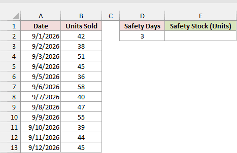
Below I have a dataset of daily ceramic coffee mug sales, and I want to keep enough extra mugs for 3 days of sales.
I have dates from 9/1/2026 to 9/12/2026 in A2:A13 and units sold in B2:B13. D2 contains 3 safety days; E2 is where the safety stock goes.
Here is the formula to enter in E2:
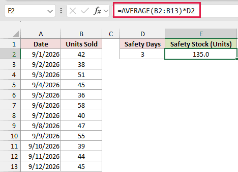
=AVERAGE(B2:B13)*D2
How does this formula work?
I use AVERAGE(B2:B13) to calculate average daily sales of 45 mugs. Multiplying by the 3 safety days in D2 returns 135 mugs, shown as 135.0 in E2.
If you change D2 to 5, you’ll get 225 mugs of safety stock.
You’re picking the cushion yourself here, so it ignores how much sales and deliveries actually swing.
Method #2: Using the Average-Max Formula
Here I look at your busiest sales day and slowest delivery instead of picking a number of extra days yourself.
The number of days between placing an order with your supplier and receiving it is called lead time.
I multiply your highest daily sales by the longest delivery wait, then subtract what you normally sell during an average wait. You don’t need statistics here.
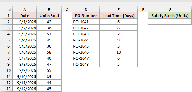
Below I have a dataset of daily ceramic coffee mug sales alongside past supplier orders. I want a buffer for the worst sales and delivery combination.
For sales, you’ll use B2:B13. The purchase orders PO-1041 to PO-1048 are in D2:D9, with delivery days in E2:E9. G2 is where the safety stock goes.
Here is the formula to enter in G2:
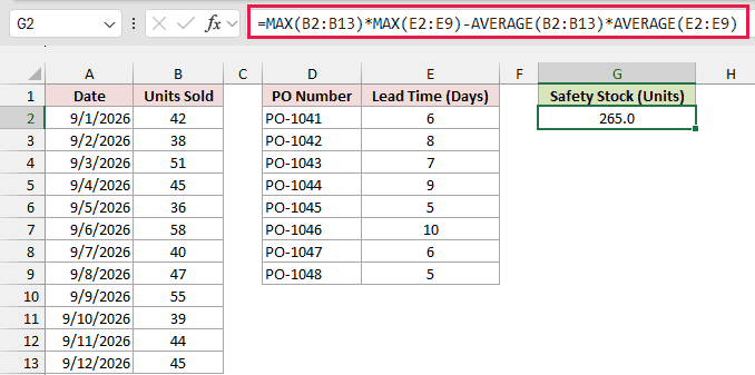
=MAX(B2:B13)*MAX(E2:E9)-AVERAGE(B2:B13)*AVERAGE(E2:E9)
How does this formula work?
The worst combination needs 580 mugs. I calculate it with MAX(B2:B13)*MAX(E2:E9), multiplying the highest daily sales, 58 mugs, by the longest wait, 10 days.
That assumes you’d repeat your busiest sales day, 9/6/2026, every day while waiting as long as your slowest delivery, PO-1046.
For your usual sales during the wait, AVERAGE(B2:B13)*AVERAGE(E2:E9) multiplies 45 mugs per day by 7 days. That’s the 315 mugs you’d normally sell before delivery.
Subtracting 315 from 580 leaves 265 mugs of extra stock. You’ll see 265.0 in G2.
Note: You’re assuming your busiest sales and slowest delivery happen together. That gives a bigger cushion here: 265 mugs versus 140.2 with Method #5. It can suit you when running out is very costly, but you’ll tie up more cash in stock.
Method #3: Using NORM.S.INV and STDEV.S (Sales Variability)
If your supplier delivers reliably but daily sales jump around, I use this formula to size the buffer from those sales swings.
To measure how far daily sales usually move from the average, I use a single number called the standard deviation. Here, it’s 6.81 mugs.
You also decide how often you want enough stock during the delivery wait. That target percentage is called your service level.
At 95%, you’d expect to run out in about 1 order cycle in 20 under the formula’s assumptions.
To turn that percentage into a multiplier, I use NORM.S.INV. The multiplier is called a Z-score; at 95%, it’s 1.645.
I multiply that by the daily sales standard deviation and the square root of the average delivery wait.
Below I have a dataset showing daily ceramic coffee mug sales and the delivery times for past orders. I want a sales buffer at a 95% service level.
Your daily sales history is in B2:B13, with delivery days in E2:E9. For the calculation, G2 holds 95%, and H2 is where the safety stock goes.
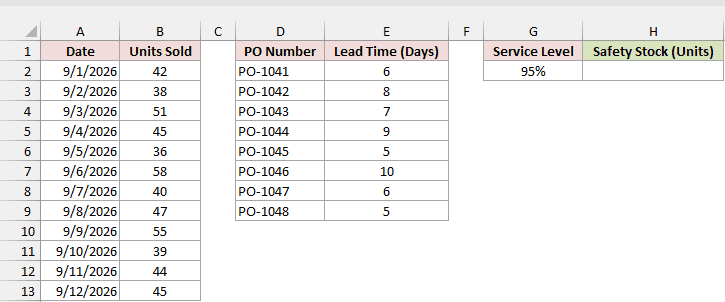
Here is the formula to enter in H2:
=NORM.S.INV(G2)*STDEV.S(B2:B13)*SQRT(AVERAGE(E2:E9))
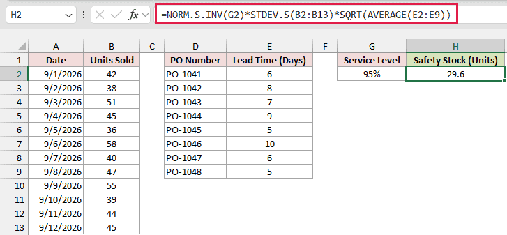
How does this formula work?
To get the multiplier for your 95% service level, I use NORM.S.INV(G2). It returns 1.645.
STDEV.S(B2:B13) returns 6.81 mugs. That measures how much your daily sales usually swing around the average.
Next, SQRT(AVERAGE(E2:E9)) returns about 2.65, the square root of your average 7-day delivery wait.
I use the square root because sales swings across several days partly cancel out. The risk grows more slowly than the number of days.
Multiplying those parts returns 29.6 mugs in H2. Excel uses the full values, so multiplying the rounded figures above gives only an approximation.
You’ll get a small buffer because I’m treating every delivery as taking exactly the average 7 days. You’re covering sales swings only.
You can use NORM.S.INV and STDEV.S in Excel 2010 and later. In older files, NORMSINV and STDEV return the same results here.
Method #4: Using NORM.S.INV and STDEV.S (Lead Time Variability)
Now I flip the assumption: your sales are steady, but your supplier’s delivery times jump around.
Here I measure the days between ordering and receiving mugs, called lead time. I want extra stock for delivery waits that run longer than usual.
I multiply the service-level multiplier by average daily sales and the standard deviation of delivery days.
Below I have a dataset pairing daily ceramic coffee mug sales with delivery days for past supplier orders. I want a delivery buffer at a 95% service level.
You can calculate average sales from B2:B13 and delivery variation from E2:E9. Your 95% service level is in G2. H2 is where the safety stock goes.
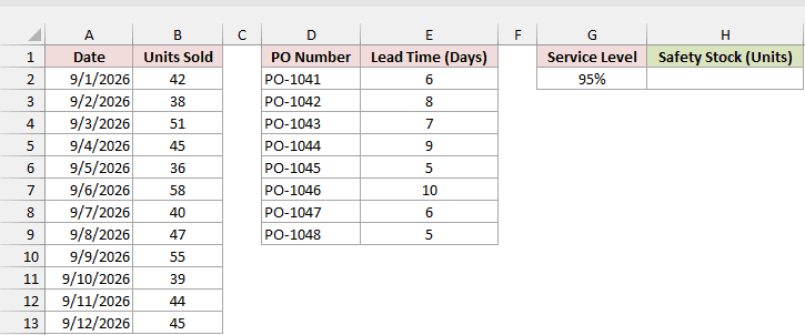
Here is the formula to enter in H2:
=NORM.S.INV(G2)*AVERAGE(B2:B13)*STDEV.S(E2:E9)
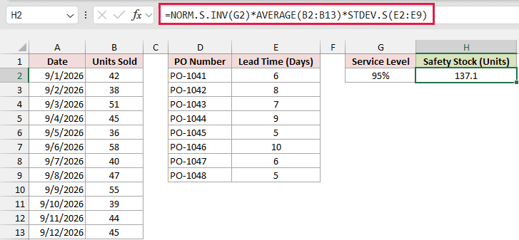
How does this formula work?
Here, NORM.S.INV(G2) returns 1.645 for your 95% service level, and AVERAGE(B2:B13) returns 45 mugs sold per day.
To measure how far delivery times usually move from the 7-day average, I use STDEV.S(E2:E9). That standard deviation is 1.85 days.
Multiplying those parts returns 137.1 mugs in H2.
When a delivery is late, you have more days of sales to cover. That’s why I multiply the delivery-time swing by daily sales.
You’ll get much more stock than Method #3 because delivery delays have a bigger effect on this buffer than sales swings.
A delivery about 1.85 days late means roughly 83 extra mugs of sales. Sales swings over the 7-day wait account for about 18 mugs.
Method #5: Using a Combined Formula (Sales and Lead Time)
In real life, both sales and delivery times can change. Here I combine the risks covered separately in Methods #3 and #4.
If you have both daily sales and delivery history, this is the formula I recommend.
You combine the risks inside a square root when sales swings and delivery delays are independent. That gives less stock than adding the separate buffers together.
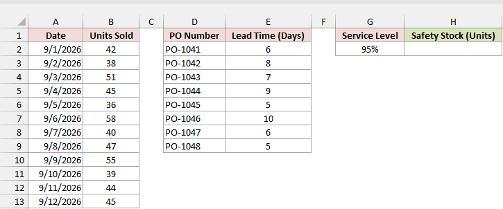
Below I have a dataset with daily ceramic coffee mug sales and past supplier delivery times. I want to cover both risks at a 95% service level.
You’ll combine the sales in B2:B13 with the delivery days in E2:E9, using 95% in G2. H2 is where the combined safety stock goes.
Here is the formula to enter in H2:
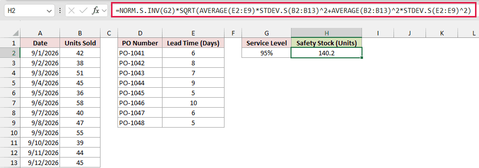
=NORM.S.INV(G2)*SQRT(AVERAGE(E2:E9)*STDEV.S(B2:B13)^2+AVERAGE(B2:B13)^2*STDEV.S(E2:E9)^2)
How does this formula work?
I calculate the sales risk with AVERAGE(E2:E9)*STDEV.S(B2:B13)^2: your average 7-day wait multiplied by the daily sales standard deviation squared, about 6.81 squared.
For delivery risk, AVERAGE(B2:B13)^2*STDEV.S(E2:E9)^2 multiplies your average daily sales squared, 45 squared, by the delivery standard deviation squared, about 1.85 squared.
I add those squared-mug amounts inside SQRT(...). The square root converts the total back into mugs, about 85.2.
Finally, NORM.S.INV(G2) scales that number to your 95% service level. You’ll see 140.2 mugs of safety stock in H2.
If you added the separate results, you’d get 29.6 + 137.1 = 166.7 mugs. The combined formula returns 140.2.
You’re allowing for both risks without assuming a sales spike and a late delivery always hit together.
Which Safety Stock Method Should You Use?
Pick the method that fits the history you have and what usually makes you run out:
| Method | What You Need | Result in This Example | Best For |
|---|---|---|---|
| Fixed safety days | Average daily sales and a number of days you pick | 135.0 | Quick estimates, new products with little history |
| Average-max | Highest and average daily sales, longest and average lead time | 265.0 | When running out is very costly and you want a big cushion |
| Sales variability | Daily sales history, average lead time, service level | 29.6 | Reliable suppliers, sales that swing |
| Lead time variability | Average daily sales, lead time history, service level | 137.1 | Steady sales, unreliable deliveries |
| Combined | Both histories and a service level | 140.2 | Most real situations (recommended) |
With both histories available, I’d use the combined formula. If you’re just getting started, fixed safety days give you a rough estimate to work with.
How to Calculate Safety Stock for Multiple Products
When you track many products, you usually have each product’s averages and standard deviations in a summary table. You can use the Method #5 formula on each row.
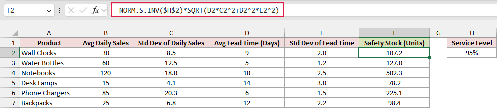
Below I have a dataset summarizing sales and delivery history for several products, and I want to calculate safety stock for each at a 95% service level.
You’ll find average daily sales in column B and daily sales standard deviation in C. Average delivery days are in D, and delivery standard deviation is in E.
H2 contains the 95% service level. F2:F7 is where the safety stock results go.

Here is the formula to enter in F2:
=NORM.S.INV($H$2)*SQRT(D2*C2^2+B2^2*E2^2)
You’ll get 107.2 for Wall Clocks. This formula doesn’t spill because it calculates one row at a time.
That per-row formula works in Excel 2010 and later. Copy it down to F7 by dragging the fill handle or double-clicking it.
How does this formula work?
I use the same combined formula as Method #5, but point it at your summary columns instead of calculating averages and standard deviations from the histories.
The dollar signs in $H$2 lock the service level cell. When you copy the formula down, every product uses the same 95% target.
You’ll get these safety stock amounts:
- Wall Clocks: 107.2 units.
- Water Bottles: 127.0 units.
- Notebooks: 502.3 units.
- Desk Lamps: 78.2 units.
- Phone Chargers: 225.1 units.
- Backpacks: 98.4 units.
You’ll need the biggest buffer for Notebooks, at 502.3 units. They sell the most, 120 a day, and their delivery times vary by about 2.5 days.
Additional Notes About Calculating Safety Stock in Excel
- Keep your time units consistent. Pair daily sales with delivery times in days, or weekly sales with weeks. Mixing them gives a wrong answer without an error.
- Round up to whole units. You can’t stock 0.2 of a mug, so
=ROUNDUP(H2,0)turns 140.2 into 141 mugs. - Use STDEV.S for a sales history like this. STDEV.P treats your data as the entire population and returns a smaller spread: 6.52 instead of 6.81 here.
- Recalculate every few months or after a big change, such as a new supplier or seasonal product. Your buffer depends on the history you’re using.
- The statistical formulas assume sales are roughly bell-shaped. If your products sell in rare, lumpy bursts, treat the result as a starting point.
Frequently Asked Questions
Once you’ve calculated the buffer, you can use it to decide when to order and how much protection you want.
How Do I Calculate the Reorder Point in Excel?
Safety stock is your extra buffer. The reorder point includes that buffer and tells you the stock level at which to order.
To calculate the reorder point, add safety stock to what you expect to sell during the delivery wait.
With the Method #5 mug data, use =AVERAGE(B2:B13)*AVERAGE(E2:E9)+H2.
Adding 315 and 140.2 returns 455.2, so you’d reorder when stock drops to about 456 mugs.
What Z-Score Should I Use for Safety Stock?
You can turn your target service level into a Z-score with NORM.S.INV. Common choices are:
- 90% service level: 1.28.
- 95% service level: 1.645, using
=NORM.S.INV(0.95). - 99% service level: 2.33.
Choose a higher percentage to run out less often, but you’ll need more stock. Changing G2 from 95% to 99% raises Method #5’s buffer to 198.3 mugs.
Conclusion
I showed you five ways to calculate safety stock in Excel, plus how to apply the combined formula to multiple products.
When you have both sales and delivery histories, Method #5 is my default for a buffer that accounts for variation in both.
Other Excel articles you may also like:
