Apply Comma Style Number Format in Excel (3 Easy Ways)

The comma style is quite commonly used when people work with financial data in Excel.

It helps improve the readability of your data as it adds commas between digits (and also adds decimals).

In this tutorial, I will show you how to quickly apply the comma style in Excel using a couple of different methods (including a keyboard shortcut).

I will also show you how you can customize the format and increase or decrease the number of decimal places in the numbers.

Table of Contents

How to Apply Comma Style in Excel

Let’s have a look at a couple of ways to apply the comma style to your data in Microsoft Excel (including a keyboard shortcut).

Using the Ribbon in Excel

Below I have a data set where I have month names in column A and the sales figures in column B, and I want to show the sales figures data with a comma-style applied to the numbers.

Here are the steps to do this:

Click the Home tab
In the Number group, click on the ‘Comma Style’ icon (the big black comma icon)

That’s it!

The comma style format would be applied to the selected cells.

When you apply a comma-style format to cells that contain numbers, you notice a few things change:

The numbers are now separated by commas. The grouping of the numbers (i.e., numbers between the commas) depends on your regional settings. This can be changed and we’ll see how to do that later in this tutorial)
A decimal point is added and two digits are added after the decimal point

If you do not want the decimal numbers in your data set, you can remove these by clicking on the Home tab and then clicking on the Decrease Decimal icon (it’s right next to the Comma Style icon)

And in case you want to increase the number of digits after the decimal point, you can use the increase decimal icon

Keyboard Shortcut to Apply the Comma Style

If you would rather prefer to use a keyboard shortcut to apply the comma-style format to your data set, you can use the below keyboard shortcut:

ALT + H + K

You need to press these keys in succession, i.e., one after the other.

Using the Format Cells Dialog Box

Another method to apply comma formatting to your data set is by using the Format Cells dialog box.

While the previous method of using the ribbon or the keyboard shortcut is faster, with the Format Cells dialog box, you get a little more control over the formatting that you can apply.

Below are the steps to apply comma style to a data set using the Format Cells dialog box:

Select the cells on which you want to apply the comma-style format
Right-click on the selection
Click on Format Cells. This will open the Format Cells dialog box

In the Format cells dialog box, select the Number tab (if not selected already)

Select the number tab in Format cells dialog box

In the Category list, select Number
Check the ‘Use 1000 separator’ option

[Optional] Change the number of decimal places

One additional option that you get when you use the Format Cells dialog box is the ability to apply red color to cells with negative values.

You can choose any of the four options in the ‘Negative Numbers; box. This allows you to show negative values in red color with or without the minus sign.

Using the Cells Styles Option

Another quick way to apply comma style in your data set is by using the styles option in Excel.

Below are the steps to use cell styles to apply comma style on your data set:

Select the cells that have the numbers on which you want to apply the comma style
Click the Home tab

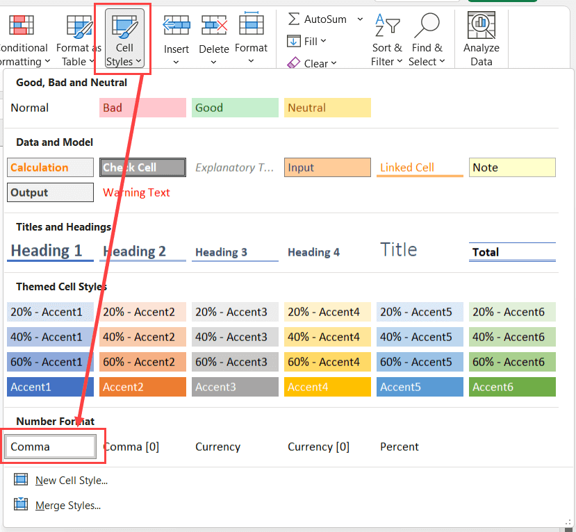
In the Styles group, click on ‘Cell Styles’
From the options that show up, click on the ‘Comma’ option in ‘Number Format’

One benefit you can get from using the Cell Styles options is that you can create your own cell style that can be applied with a single click.

For example, if in addition to applying the comma style, you also want the cells to have a specific type of border or fill color or alignment/font, you can create a new style and specify all these formattings to it.

This can be done using the ‘New Style’ option that shows up when you click on the ‘Cell Styles’ option in the ‘Home’ tab.

Once you have created a new style, you can easily apply it to any cell by going to the Cell Styles options and clicking on that style (it would show up in the options once you create it)

Changing the Comma to Decimal in Numbers (or Vice Versa)

In many regions, there’s a difference in the way numbers are shown.

For example, in South America and some European countries, a decimal is used instead of a comma, and a comma is used instead of a decimal.

To give you an example, instead of 12,34,567.00, the format would be 12.34.567,00

While Excel is smart enough to take care of the formatting when you share your Excel file with someone who has the regional setting that uses decimal instead of a comma, let me still show you a method that will allow you to make this change on your system.

Below are the steps to change the comma to decimal in Excel:

Click the Home tab
Click on Options
In the Excel Options dialog box, select Advanced

In the ‘Editing’ options, uncheck ‘Use system separators’
Change the Decimal Separator to comma (,)
Change the Thousands separator to decimal point (.)

Click Ok

The above steps would turn off your system’s in-built setting, and use the separators that you have specified.

In this example, I have simply interchanged a decimal point and a comma, but you can also use other separators if you want.

Also note that this does not change the number in the back end, and only changes the way the numbers are being displayed to the user.

If you want to revert these changes and get the default setting back, open the Excel Options dialog box and check the ‘Use system separators’

How to Change Comma Style from Lakhs to Millions in Excel?

Different regions have different ways of comma styles that they apply to numbers.

For example, in the US and UK, a comma is placed after every third digit (when going from left to the right). So, 1 million would be 1,000,000

On the other hand, another popular comma style method is using Lakhs and Crores, where a comma is placed after the first three digits (considering left to right) and then every second digit.

So, 1 million would be 10,00,000

If you have the lakh comma style and you want to change it to the million comma style, you can do that by using the steps below:

Go to the Control Panel in your system (you can search for it in the search bar)
Click on the ‘Change date, time, or number format’ option

In the Region dialog box that opens up, click on the Additional Settings button. This will open the Customize Format dialog box.

Click on the Currency tab

In the ‘Digit grouping’ dropdown, select the million comma style

Select the million comma format grouping

Click on Apply

Once the above changes are done, all the numbers would be displayed in the million, style format.

In case you want to revert to the original default settings, you can do that by clicking on the Reset button in the Currency tab in the Customize Format dialog box.

In this tutorial, I covered three different methods to apply the comma-style format for numbers in Excel (including a keyboard shortcut).

I also covered how to interchange a comma with a decimal point in numbers (which is the accepted format in many regions), as well as the process to change the Lakh comma style format to the million comma style format.

Other Excel tutorials you may also find useful: