While strikethrough is mostly used in Office applications such as Microsoft Word or Outlook, a lot of users also use it in Excel.
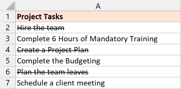
One common use case where you may want to show completed tasks with a line across the text to indicate that it has been completed (as shown below)
Since strikethrough is not such a commonly used feature in Excel, you won’t be able to find it in the ribbon. It’s available in Excel, but you got to know where to find it.
In this tutorial, I will show you some easy methods you can use to quickly apply strikethrough formatting on cells in Excel (including a keyboard shortcut to apply strikethrough)
Strikethrough Keyboard Shortcut in Excel
Let’s start with the easiest way to apply strikethrough format on a cell in Excel – a keyboard shortcut.
Below is the keyboard shortcut for strikethrough in Excel (Windows):
Control + 5
To use the shortcut, hold the Control key and then press the 5 key.
And if you’re using a Mac OS, here is the keyboard shortcut for strikethrough:
Cmd+Shift+X
To use this, hold the Command and the Shift key and then press the X key.
The keyboard shortcut would work as a toggle, so if you use it once it would apply the strikethrough format on a cell, and if you use it again it would remove it.
If you select a range of cells and then use this keyboard shortcut, the strikethrough format would be applied to all the cells.
Bonus Tip: This strikethrough keyboard shortcut also works in Google Sheets
Add Strikethrough Icon to Quick Access Toolbar
If you’re not a fan of using keyboard shortcuts in Excel, or you already have a lot of keyboard shortcuts that you need to memorize and don’t want another one, let me show you another quick way to apply the strikethrough format in Excel.
You can add the strikethrough format icon in the Quick Access Toolbar (QAT) so that it’s always visible and you can use it with a single click whenever you want.
Below are the steps to add the strikethrough format icon in the Quick Access Toolbar:
- Click on the ‘Customize the Quick Access Toolbar’ icon

- Click on ‘More Commands’

- In the ‘Excel Options’ dialog box that opens up, click on ‘Choose commands from ‘ drop-down
- Choose the ‘Command Not in the Ribbon’ option

- Scroll down and select the Strikethrough option in the commands box. The commands are listed in alphabetical order, so you need to scroll toward the end of the list

- Click on the Add button

- Click Ok

The above steps would add this strikethrough icon in the Quick Access Toolbar.
To use this, first, select the cells where you want to apply the strikethrough format, and then click on the strikethrough icon in the QAT.
It works as a toggle, so clicking it once would apply the strikethrough format, and clicking it again would remove it.
Also read: How to Remove Strikethrough in Excel?
Strikethrough Using Format Cells Dialog Box
Another way to apply strikethrough format in Excel is by using the format cells dialog box.
Although this is a longer method (compared with the keyboard shortcut or using the strikethrough option in the Quick Access Toolbar) the benefit of this method is that it allows you access to more options that you can use along with the strikethrough format.
Below are the steps to apply the strikethrough formatting excel using the Format Cells dialog box:
- Select the cells on which you want to apply the strikethrough format
- Click the ‘Home’ tab

- In the Font group, click on the dialog box launcher (the small arrow at the bottom right part of the group)

- In the Font tab, check the Strikethrough option

- Click OK
The above steps would apply the strikethrough format to the content of the selected cell.
As I mentioned, you get access to more options in the Format Cells dialog box (such as changing the font, font style, font size, font color, as well as the subscript and superscript format)
Using Cell Styles to Apply Strikethrough Formatting to Cells
Another way to apply strikethrough format in Excel is by creating a cell style, and then reusing it.
This would be best for scenarios where you need to apply multiple formats (such as changing the font color along with the strikethrough).
Below are the steps to do this:
- Click the ‘Home’ tab
- In the Styles group, click on ‘Cell Styles’

- In the options that show up, click on ‘New Cell Style’

- In the Style dialog box, give a name to this style. In our example, I would name it StrikeThrough

- Click the Format button

- In the Format Cells dialog box, select the ‘Font’ tab
- Check the Strikethrough box
- [Optional] Specify any other formatting that you want to be applied to the selected cells. This could be in the Fonts tab or any other tab
- Once done, click on OK
The above steps would create a new cell style that would be available when you click on the Cell Styles option in the ribbon. It would show up under the customs group.

Once created, you can easily apply the style by selecting the cells, clicking on the cell styles option in the home tab, and then clicking on the newly created style.
Note that any style that you create would be localized to the workbook, and would not be available to any other workbook that you opened on your system.
However, you have the option to ‘Merge Styles’, so in case you already have a workbook that has a custom style made, you can merge that style with your current workbook and get access to it.
Strikethrough Using Conditional Formatting
And the last method that I want to show you to apply strikethrough in Excel is by using Conditional Formatting.
Conditional formatting works by analyzing the value in the cell, and if the specified condition is met, then it applies the specified formatting.
Below I have an example data set, where I have some tasks in column A, and their status in column B.

I can use conditional formatting in such a way that whenever the status is entered as completed in column B, the task in column A would be stricken-off.
Below are the steps to do this:
- Select the cells that contain the tasks and column A

- Click the ‘Home’ tab
- In the Styles group, click on ‘Conditional Formatting’

- In the options that show up, click on ‘New Rule’

- In the New Formatting Rule dialog box, click on the ‘Use a formula to determine which cells to format’ option

- Enter the below formula in the formula field
=B2="Completed"

- Click on the Format button

- In the ‘Format’ cells dialog box, click on the ‘Font’ tab
- Check the Strikethrough option
- Click OK
- Click OK

The above steps would apply the strikethrough format on all the tasks where the status is mentioned as completed.

Also note that conditional formatting is dynamic, so if you change the status from completed to something else, the strikethrough format would be removed.
Let me also quickly explain what happens here.
When we selected the cells in column a comma and used the formula =B2=”Completed” in Conditional Formatting, each cell in the selection is now assessed using this formula.
For cell A1, the formula that’s used is
=B2=”Completed”
For cell A2, the formula is
=B3=”Completed”
And so on..
So for each task in column A, the value in the adjacent column is analyzed, and if that value is “Completed”, the strikethrough format is applied on that task, else it’s not.
Can You Apply Strikethrough to Partial Text in a Cell?
Yes, you can apply the strikethrough format in a cell partially, which means that some parts of the cell content would be stricken-off, and the rest won’t (as shown below).

To do this, follow the below steps
- Double-click on the cell in which you want to apply the strikethrough format (or select the cell and hit the F2 key to get into the edit mode)
- Select the text on which you want to apply the strikethrough format
- Use the keyboard shortcut Control + 5 (or use a strikethrough icon in the Quick Access Toolbar or Format Cells dialog box)
The above steps would only apply the strike-off only the cell content that was selected.
Also read: Excel Fill Color Shortcut
How to Change Strikethrough Color in Excel?
A common question for many people who want to apply the strikethrough format in Excel is whether you can have a different color for the strikethrough line and a different color for the text behind it.
For example, many people want the text to be in black color, but the strikethrough line in red color.
Unfortunately, this is not something that can be done in Excel. When you apply a format on a cell (such as font size or font color), it is applied to the entire cell.
However, if you still need to have a separate color for the strikethrough line, there is a workaround.
You can use the Shapes option to insert a line over the text manually and then give any color you want to that line.
It’s not an elegant solution, and should only be used if you absolutely need this.
Below are the steps to insert a line and then give it a different color:
- Click the Insert tab

- Click on Illustrations

- Click on Shapes

- Click on the Line that you want to insert into the worksheet

- Bring the cursor to the worksheet, hold the left mouse key, and drag it to insert the line
- Place the line over the text where you want to show it as a strikethrough

- With the line selected, click on the ‘Shape Format’ tab
- Click on the Shape Outline option, and then select the color for the line (and also change the weight of the line in case it looks thin)

Once the line is added for one cell, copy the line and place it over other cells where you want to show a strike-off in a different color.

As I mentioned, this is not an elegant solution, and if you need to do this for multiple cells, you would have to insert the line multiple times.
In this tutorial, I showed you a few different ways to insert the strikethrough format in Excel.
The fastest way would be to use the keyboard shortcut or add the strikethrough icon in the Quick Access Toolbar and then click on it to apply that.
And if you work with task lists and project status reports, you can also use the strikethrough format to visually show tasks that have been completed by using Conditional Formatting.
I hope you found this Excel tutorial helpful.
Here are some other Excel tutorials you may also find useful:
- How to Add Bullet Points in Excel
- How to Apply Comma Style Number Format in Excel
- How to Paste without Formatting in Excel (Shortcuts)
- How to Copy Formatting In Excel
- How to Auto Format Formulas in Excel
- How to Highlight Every Other Row in Excel (Conditional Formatting & VBA)
- Subscript in Excel
- Superscript in Excel
- Insert Checkmark in Excel (Shortcut)
- How to Insert Degree Symbol in Excel?
- How to Filter Strikethrough in Excel