
Cell Styles let you give titles, totals, inputs, warnings, and other worksheet elements consistent formatting without rebuilding that formatting one piece at a time.
A style can control the font, fill, border, alignment, number format, and protection settings. Apply another style later, and Excel replaces those settings as a group.
I’ll show you how to apply the common named styles first, then create, change, copy, remove, delete, and merge styles between workbooks.
Note: These instructions were verified in Microsoft 365 for Windows desktop. The Mac and Excel for the web versions were not tested.
What Cell Styles Are and Why They Beat Manual Formatting
Manual formatting changes one setting at a time. A cell style stores a named set of settings, so you can apply the whole combination in one click.
The name also gives the formatting a job. Someone opening your workbook can tell that a cell is an Input, Calculation, Total, or Note instead of guessing from its color.
Styles belong to the workbook. Changing a style updates every cell using it in that workbook, which is useful when a report needs a consistent redesign.
Method #1: Applying a Built-In Cell Style
This is the method I recommend for most readers. Excel already includes styles for the worksheet elements you’re likely to format.
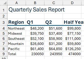
Below, I have a quarterly sales sheet with a report title, column headings, calculation cells, and a total row.
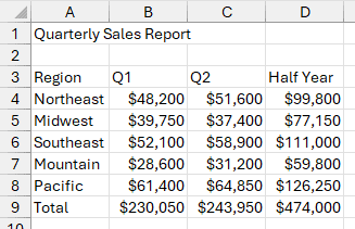
Here are the steps to apply a built-in cell style:
- Select the cell or range you want to format. On the Home tab, open Cell Styles in the Styles group.
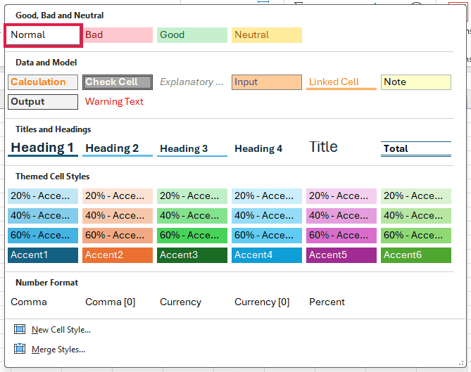
- Click the style you want to apply.
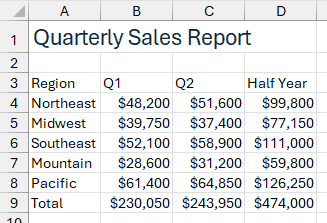
Excel applies every formatting component included in that style. You can repeat the same steps for another cell or choose another style for the current selection.
Applying the Most-Searched Cell Styles
Coursework instructions often name one exact style and one target cell. Select that cell first, then use the matching entry below.
Applying the Title Cell Style
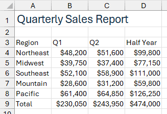
Select the title cell, then go to Home > Cell Styles > Title. Title uses Aptos Display at 18 points with dark text, and it is not bold.
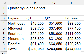
Applying the Total Cell Style
Select the cells in your total row, then go to Home > Cell Styles > Total. Excel adds bold text, a top rule, and a double bottom rule.
Applying Heading 1, 2, 3, and 4
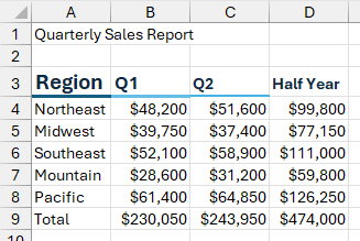
Select a heading cell, open Cell Styles, and choose Heading 1, Heading 2, Heading 3, or Heading 4.
The borders get progressively lighter. Text size drops from 15 to 13 to 11 points, then stays at 11 points for Heading 4.
Applying the Calculation Cell Style
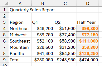
Select the formula cell, then choose Calculation from Cell Styles. This style uses bold orange text, a light fill, and a boxed border with a double top.
Applying the Accent 1 Cell Style
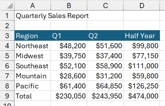
Select the cells, then choose Accent 1 from Cell Styles. Its color comes from the workbook theme, so the same style can look different under another theme.
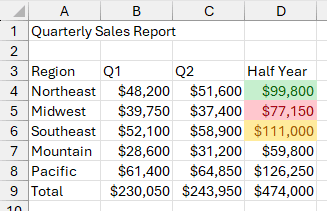
Applying Good, Bad, and Neutral Cell Styles
Select the result cells, then choose Good, Bad, or Neutral from Cell Styles. These styles use colored text and fills, but none is bold or bordered.
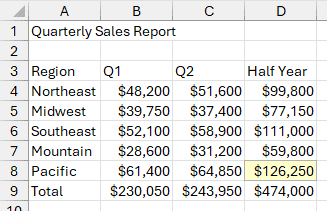
Applying the Note Cell Style
Select the cell containing your note, then choose Note from Cell Styles. Excel applies a pale yellow fill and a thin box border.
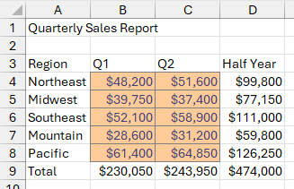
Applying the Input Cell Style
Select the cells where users should type, then choose Input from Cell Styles. The orange fill, dark text, and thin border make entry cells easy to spot.
Full List of Built-In Cell Styles in Excel
The table below lists all 47 styles found in the default gallery on the tested Microsoft 365 installation.
The accent colors shown here reflect the current Office theme. Themed Cell Styles change when you change the workbook’s theme colors.
| Gallery group | Cell style | Formatting applied |
|---|---|---|
| Good, Bad and Neutral | Normal | Aptos Narrow 11-point black text, no fill, no border, and not bold |
| Good, Bad and Neutral | Bad | Dark red text (#9C0006) on a light red fill (#FFC7CE), no border, and not bold |
| Good, Bad and Neutral | Good | Dark green text (#006100) on a light green fill (#C6EFCE), no border, and not bold |
| Good, Bad and Neutral | Neutral | Dark orange text (#9C5700) on a light yellow fill (#FFEB9C), no border, and not bold |
| Data and Model | Calculation | Bold orange text (#FA7D00) on a light gray fill (#F2F2F2), a thin gray box, and a thick double top border (#3F3F3F) |
| Data and Model | Check Cell | Bold white text on a gray fill (#A5A5A5) with a thick double border (#3F3F3F) on all four sides |
| Data and Model | Explanatory Text | Italic gray text (#7F7F7F), no fill, and no border |
| Data and Model | Input | Dark blue-purple text (#3F3F76) on an orange fill (#FFCC99) with a thin box border |
| Data and Model | Linked Cell | Orange text (#FA7D00), no fill, and a thick double orange bottom border (#FA7D00) |
| Data and Model | Note | Pale yellow fill (#FFFFCC) with a thin gray box border (#B2B2B2) |
| Data and Model | Output | Bold dark gray text (#3F3F3F) on a light gray fill (#F2F2F2) with a thin box border |
| Data and Model | Warning Text | Red text (#FF0000), no fill, and no border |
| Titles and Headings | Heading 1 | 15-point bold dark text (#0E2841) with a thick double top and thick bottom border (#156082) |
| Titles and Headings | Heading 2 | 13-point bold text with a thick top border (#156082) and a thick pale blue bottom border (#E4F2F6) |
| Titles and Headings | Heading 3 | 11-point bold text with a thick pale blue top border (#E4F2F6) and a medium teal bottom border (#44B3D4) |
| Titles and Headings | Heading 4 | 11-point bold text with a medium teal top border (#44B3D4) only |
| Titles and Headings | Title | Aptos Display 18-point dark text (#0E2841), not bold, no fill, and no border |
| Titles and Headings | Total | Bold black text, no fill, a thin top rule, and a thick double bottom rule (#156082) |
| Themed Cell Styles | Accent1 | White text on the current Accent 1 fill (#156082) |
| Themed Cell Styles | Accent2 | White text on the current Accent 2 fill (#E97132) |
| Themed Cell Styles | Accent3 | White text on the current Accent 3 fill (#196B24) |
| Themed Cell Styles | Accent4 | White text on the current Accent 4 fill (#0F9ED5) |
| Themed Cell Styles | Accent5 | White text on the current Accent 5 fill (#A02B93) |
| Themed Cell Styles | Accent6 | White text on the current Accent 6 fill (#4EA72E) |
| Themed Cell Styles | 20% – Accent1 | Black text on a 20% tint of Accent 1 |
| Themed Cell Styles | 20% – Accent2 | Black text on a 20% tint of Accent 2 |
| Themed Cell Styles | 20% – Accent3 | Black text on a 20% tint of Accent 3 |
| Themed Cell Styles | 20% – Accent4 | Black text on a 20% tint of Accent 4 |
| Themed Cell Styles | 20% – Accent5 | Black text on a 20% tint of Accent 5 |
| Themed Cell Styles | 20% – Accent6 | Black text on a 20% tint of Accent 6 |
| Themed Cell Styles | 40% – Accent1 | Black text on a 40% tint of Accent 1 |
| Themed Cell Styles | 40% – Accent2 | Black text on a 40% tint of Accent 2 |
| Themed Cell Styles | 40% – Accent3 | Black text on a 40% tint of Accent 3 |
| Themed Cell Styles | 40% – Accent4 | Black text on a 40% tint of Accent 4 |
| Themed Cell Styles | 40% – Accent5 | Black text on a 40% tint of Accent 5 |
| Themed Cell Styles | 40% – Accent6 | Black text on a 40% tint of Accent 6 |
| Themed Cell Styles | 60% – Accent1 | Black text on a 60% tint of Accent 1 |
| Themed Cell Styles | 60% – Accent2 | Black text on a 60% tint of Accent 2 |
| Themed Cell Styles | 60% – Accent3 | Black text on a 60% tint of Accent 3 |
| Themed Cell Styles | 60% – Accent4 | Black text on a 60% tint of Accent 4 |
| Themed Cell Styles | 60% – Accent5 | Black text on a 60% tint of Accent 5 |
| Themed Cell Styles | 60% – Accent6 | Black text on a 60% tint of Accent 6 |
| Number Format | Comma | Accounting format with two decimal places |
| Number Format | Comma [0] | Accounting format with no decimal places |
| Number Format | Currency | Accounting format with a currency symbol and two decimal places |
| Number Format | Currency [0] | Accounting format with a currency symbol and no decimal places |
| Number Format | Percent | Percentage number format |
Despite their names, the Comma and Currency styles use Accounting formatting. That puts the symbol at the cell edge and shows negatives in parentheses and zero as a dash.
The Currency styles therefore behave like the Accounting number format, not the standard Currency format.
Hyperlink and Followed Hyperlink can also appear after the workbook contains a hyperlink. A Custom group appears at the top after you create a custom style.
Method #2: Creating a Custom Cell Style
If the built-in choices do not match your workbook, create a named style containing only the settings you want.
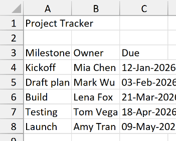
Below, I have a project tracker with milestone cells that need the same font, fill, and border throughout the workbook.
Here are the steps to create a custom cell style:
- Go to Home > Cell Styles > New Cell Style. Enter a name for the style, then click Format.
- Choose the formatting in the Format Cells dialog and click OK. Clear any unwanted boxes under Style Includes, then click OK again.
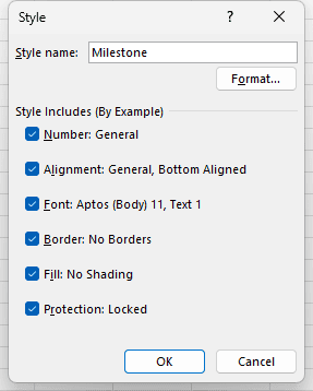
The new style appears in a Custom group at the top of the gallery. It is available only in the current workbook unless you merge it or use a template.
Method #3: Modifying a Built-In Cell Style
Here’s another way to change several formatted cells at once. Modify the style itself instead of editing each cell.
Suppose your expense report has several totals already using the Total style.
Here are the steps to modify the style:
- Open Cell Styles, right-click the style, and choose Modify. There is no separate Edit command.
- Click Format, change the required settings in Format Cells, then click OK in both dialogs.
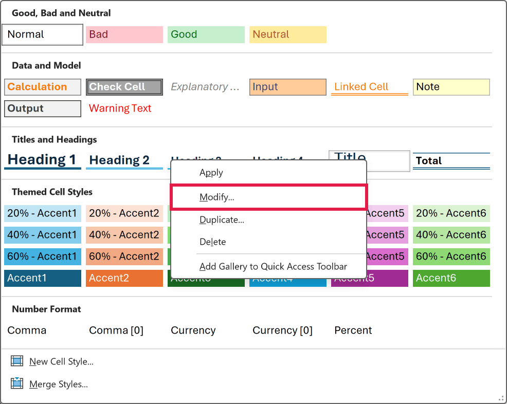
Every cell using that style updates immediately in the current workbook. If you want a variation without changing existing cells, duplicate the style instead.
Method #4: Duplicating a Cell Style
Duplicating is the safer choice when an existing style is close to what you need, but its current cells must stay unchanged.
Suppose your budget sheet uses Input cells and you need a similar style for optional inputs.
Here are the steps to duplicate the style:
- Open Cell Styles, right-click the original style, and choose Duplicate. Enter a new name, click Format, make the changes, and click OK.
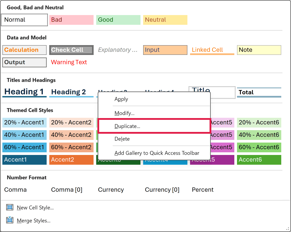
The duplicate appears in the Custom group. Cells using the original style remain unchanged.
Method #5: Removing a Cell Style From Cells
Use the Normal style when selected cells should return to the workbook’s standard cell appearance.
Below, I have status cells using the Good style, and I want to remove that green formatting.
Here are the steps to remove the style:
- Select the cells, open Cell Styles, and choose Normal.
Normal replaces the selected cells’ current formatting with the Normal definition. It does not peel away only the named style while preserving manual changes.
Method #6: Deleting a Cell Style From the Workbook
Deleting removes the style definition from the workbook, not only from the selected cells. Check where the style is used before doing this.
Suppose your workbook has an old custom Review style that you no longer need.
Here are the steps to delete the style:
- Open Cell Styles, right-click the style, and choose Delete.
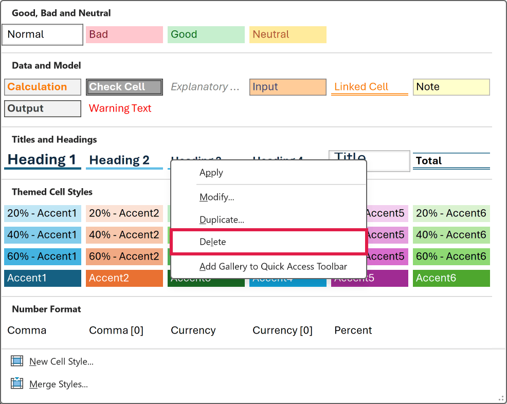
Excel lets you delete built-in styles too. Cells that used the deleted style revert to Normal.
Method #7: Merging Cell Styles From Another Workbook
Merging is the quickest way to bring a set of workbook-local styles into another file.
Below, I have a destination report and a source workbook containing the approved custom styles. Both files are open in the same Excel instance.
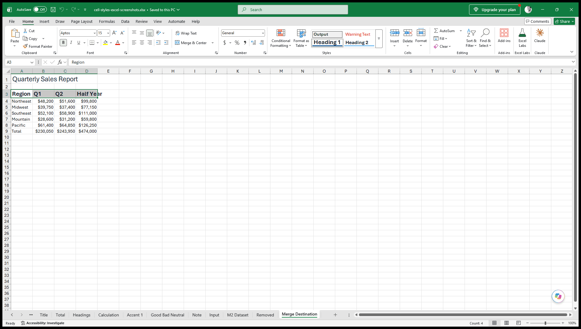
Here are the steps to merge the styles:
- In the destination workbook, go to Home > Cell Styles > Merge Styles. Choose the source workbook in the Merge styles from dialog, then click OK.
- If Excel finds matching style names, it asks once whether to replace all clashing names. Click Yes only when the source definitions should replace them.
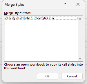
Merge Styles lists only workbooks open in the same Excel instance. To use the same styles in every new workbook, save a Book.xltx template in XLSTART, Excel’s startup folder.
Additional Notes About Cell Styles in Excel
- Changing the theme recolors theme-based styles immediately. Changing Excel’s theme colors can repaint Accent styles and alter Heading and Title font colors.
- Conditional formatting sits above a cell style. A red conditional-formatting rule can display over a Good style while the Good fill remains underneath.
- A cell style overrides an Excel Table’s banded fill for that cell. Remove the cell-level style with Normal or choose Home > Editing > Clear > Clear Formats to reveal the table formatting again.
- Applying Normal also removes direct formatting, such as a manually applied italic setting. Excel applies the complete Normal definition rather than removing only the previous style.
- There is no dedicated hotkey for an individual cell style. Alt, H, J opens the gallery, and F4 repeats the last style application.
Frequently Asked Questions
How do I apply the Total cell style to selected cells?
Select the cells, go to Home > Cell Styles, and click Total. Excel applies bold text with a top rule and a double bottom rule.
Why did my cell styles change color after I changed the theme?
Theme-based styles use the workbook’s theme colors rather than fixed colors. When you switch the theme color scheme, Excel updates those styles immediately.
Can I use my custom cell styles in another workbook?
Yes. Open both workbooks in the same Excel instance, then use Cell Styles > Merge Styles in the destination workbook.
For every new workbook, save the styles in a Book.xltx template inside XLSTART.
Why is the Cell Styles button grayed out?
The sheet may be protected without permission to format cells, the file may be in Protected View or read-only, or several worksheets may be grouped.
What is the difference between a cell style and a table style?
A cell style formats selected cells. A table style formats the whole Excel Table, including its header and banded rows.
If both affect the same cell, the cell style’s fill appears over the table banding.
Is there a keyboard shortcut to apply a cell style in Excel?
No individual style has a dedicated shortcut. Press Alt, H, J to open the gallery, use the arrow keys to choose a style, and press Enter.
F4 repeats the last style application. Ctrl+Shift+C and Ctrl+Shift+V copy and paste formatting, but they do not select a named style.
Conclusion
I showed how to apply, create, change, and share Cell Styles so repeated worksheet elements keep a consistent look. I hope you found this article helpful.
Other Excel articles you may also like:
