Excel Not Saving Formatting: Causes and Fixes

You format an Excel sheet, save it, and reopen it only to find the colors, borders, or number formats gone.

Most of the time, the cause is the file type or a setting rather than an Excel bug.

I’ll show you how to check the file format, stop refreshes from resetting your formatting, and change workbook defaults, starting with the most common cause.

Reason #1: The File Is Saved as a CSV (or Another Text Format)

This is the most common reason Excel doesn’t keep your formatting. CSV and TXT files store the text you see in cells, without the workbook’s formatting.

Bold text, fills, borders, column widths, and number formats aren’t kept. Neither are extra worksheets or formulas; formulas become their displayed results.

Below I have an invoice list in A1:F9, with a light pink, bold header row and gray borders.

The dates use a format like Sep 1, 2026, ZIP codes use 00000 to display leading zeros, and amounts use currency formatting.

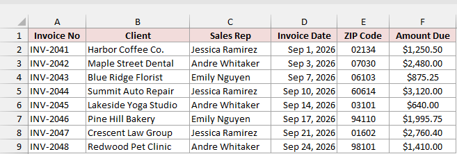
Here is the same list after I saved it as a CSV and opened it again:

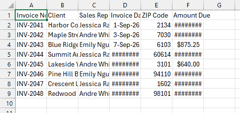
The header fill, bold text, and borders are gone. Columns have returned to their default widths, so some dates and amounts show as #####.

The ZIP codes have lost their leading zeros: 02134 became 2134, and 07030 became 7030. The first invoice date now shows as 1-Sep-26.

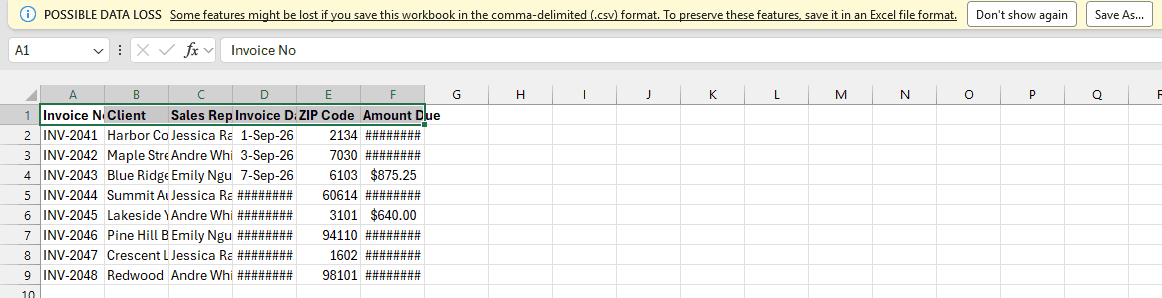
To test this, I bolded the header in the reopened CSV and pressed Ctrl+S.

When you save a CSV containing features it can’t keep, Excel displays a yellow POSSIBLE DATA LOSS message bar warning that some features might be lost.

Fix: Save the File as an Excel Workbook (.xlsx)

Use .xlsx for the file you work on so Excel can save its formatting. Here are the steps:

1. Press F12, or go to File > Save As > Browse, to open the Save As dialog.

2. In the Save as type drop-down, choose Excel Workbook (*.xlsx).

3. Click Save.

From now on, keep the .xlsx as your working file. If another system needs a CSV, save a separate CSV copy at the end.

Note: Saving a CSV as .xlsx cannot restore lost formatting. Reapply it or open an earlier .xlsx copy. Renaming the extension does not help either.

Reason #2: The Workbook Is in the Old .xls Format (Compatibility Mode)

If your file already has an Excel extension, check whether it ends in .xls. That’s the Excel 97-2003 format, which shows Compatibility Mode in the title bar.

It supports about 4,000 unique cell-format combinations, compared with about 64,000 in .xlsx. A heavily formatted workbook can reach that smaller limit.

Newer formatting, including data bars, color scales, and icon sets, can be lost or degraded when someone opens the file in Excel 2003 or earlier.

Microsoft 365 keeps those features when it saves an .xls file.

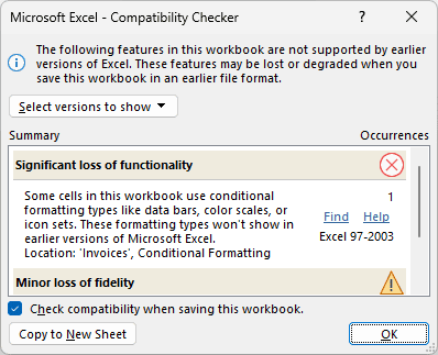
The real risks are the smaller format limit and anyone opening the file in an older version. The Compatibility Checker lists what’s at risk.

Below I have the invoice list saved as Invoices.xls, with data bars in the Amount Due column.

Go to File > Info > Check for Issues > Check Compatibility to see the issues listed in the Compatibility Checker:

Fix: Convert the Workbook to the Current Format

Converting the workbook removes the old-format restrictions.

Convert replaces the .xls file, so use Save As instead if you want to keep the original as a backup.

Here are the steps to convert it:

1. Go to File > Info and click Convert.

2. Click OK in the confirmation, then click Yes when Excel asks to close and reopen the workbook.

The workbook is now .xlsx, Compatibility Mode disappears from the title bar, and newer formatting can be saved normally in the current format.

Reason #3: You’re Editing a Read-Only Copy

If the original file looks unchanged after you save, you may be editing a read-only copy. Check for Read-Only in Excel’s title bar.

This can happen when Windows marks the file read-only, someone else has it open, or you open an email attachment.

Excel can’t save over the original in these cases. Your changes belong to the new copy you save; the original stays as it was.

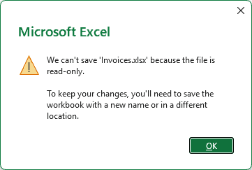
Below I have Invoices.xlsx, which is marked read-only in Windows. After formatting it, I press Ctrl+S.

Excel tells me it can’t save over the file and asks me to save a copy with a new name:

Fix: Save a Copy or Remove the Read-Only Setting

Choose the option that matches how you opened the file:

• If someone else has the file open, go to File > Save As, save with a new name, and work from that file.
• For a Windows read-only setting, close the workbook. Right-click the file in File Explorer > Properties, uncheck Read-only, click OK, and reopen it.
• For an email attachment, save the attachment to a folder first. Then open and edit that saved file.

Reason #4: A Refresh Is Resetting the Formatting

If your column widths change after a refresh, check the table’s refresh settings. PivotTables and Power Query tables rebuild themselves when refreshed.

If someone has turned off Preserve cell formatting, fills and number formats you applied also reset on refresh.

By default, PivotTables have Autofit column widths on update turned on. Power Query tables have Adjust column width turned on, so manually set widths can snap back.

I’ll show you where to change those settings for each table type.

Fix #1: Change the PivotTable Options

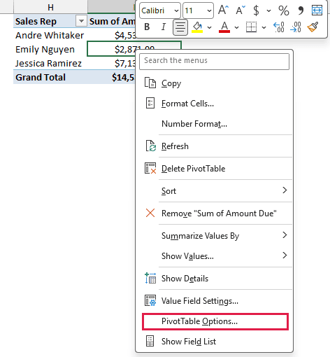
Below I have a PivotTable that sums Amount Due by Sales Rep from the invoice list.

Andre Whitaker totals $4,530.00, Emily Nguyen totals $2,871.00, and Jessica Ramirez totals $7,130.90. The Grand Total is $14,531.90.

Here are the steps to keep its column widths and cell formatting:

1. Right-click any cell in the PivotTable and choose PivotTable Options.

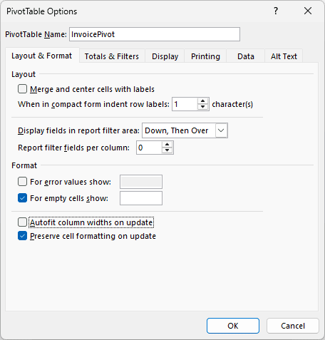
2. On the Layout & Format tab, uncheck Autofit column widths on update and make sure Preserve cell formatting on update is checked.

3. Click OK.

For PivotTable number formats, right-click a value > Value Field Settings > Number Format, rather than applying them from the Home tab.

That attaches the format to the value field so it survives layout changes.

Fix #2: Change the Query’s External Data Properties

For a Power Query table, the width setting lives in a different dialog. Below I have the same invoices loaded to a worksheet with Power Query.

Here are the steps to preserve its column widths:

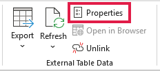
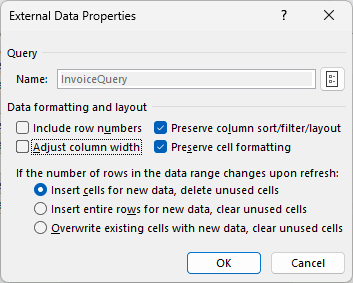
1. Click any cell in the query table, then go to Table Design > Properties in the External Table Data group.

2. In the External Data Properties dialog, uncheck Adjust column width and keep Preserve cell formatting checked.

3. Click OK.

The next refresh keeps the column widths you set.

Reason #5: Conditional Formatting Is Overriding Your Format

If only some cells refuse to show your chosen fill or font color, a conditional formatting rule may be covering it.

Conditional formatting sits on top of regular formatting. Excel can save your manual format while displaying the rule’s format instead.

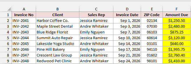
Below, the Amount Due cells in F2:F9 have a yellow fill, but three of them still show a light red fill with dark red text.

Those cells contain $2,480.00, $3,120.00, and $2,760.40:

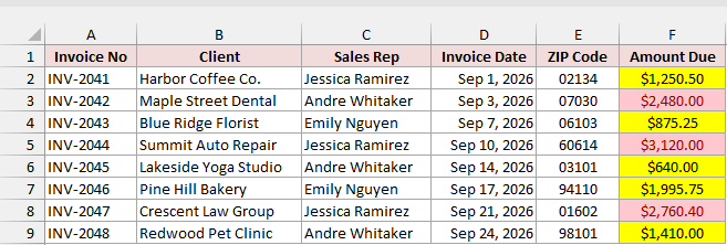
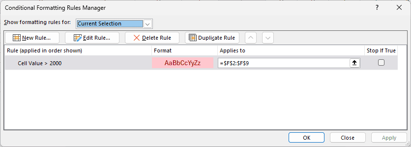
A conditional formatting rule, Cell Value > 2000, is painting over those cells because their amounts exceed $2,000.

Fix: Edit or Delete the Rule in the Rules Manager

You can remove the rule or change its formatting. Here are the steps:

1. Select F2:F9, then go to Home > Conditional Formatting > Manage Rules.

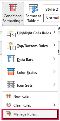
2. In the Conditional Formatting Rules Manager, select Cell Value > 2000. If you don’t see it, choose This Worksheet in Show formatting rules for. Click Delete Rule, or Edit Rule to change its format.

3. Click OK.

Once the rule is gone, the yellow fill shows in every cell in F2:F9:

Reason #6: The Workbook Has Too Many Cell Formats

If Excel shows a “Too many different cell formats” message, the workbook may have reached its limit of about 64,000 unique format combinations for .xlsx files.

Each combination includes the font, borders, fill, number format, alignment, and protection settings. Past the limit, Excel can stop applying formatting or drop it.

Years of copying sheets between workbooks can bring along leftover custom styles. Names such as Normal 2, Comma 3, and Currency 2 are common clues.

Fix: Delete Unused Styles and Clear Formatting You Don’t Need

Remove styles you don’t use and formatting outside the actual data. Here are the steps:

1. Go to Home > Cell Styles. Look in the Custom group at the top, right-click an unused style, and choose Delete. Repeat for other unused styles.

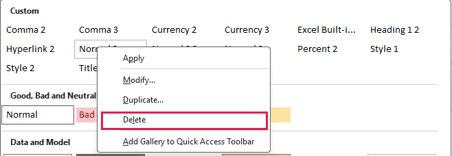
Excel doesn’t show which styles are in use. Deleting a style still in use switches those cells back to the Normal style.

Only delete styles you’re sure you don’t need.

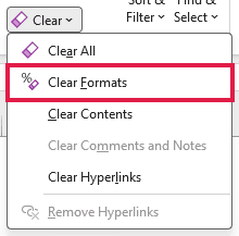
2. Select cells outside your data that carry a mix of formats. To clear the formatting, go to Home > Clear > Clear Formats. Whole rows or columns formatted by accident are common candidates.

3. Save the file.

If your Excel has the Inquire tab (Microsoft 365 Apps for enterprise and some Office Professional Plus versions), Clean Excess Cell Formatting does the clearing for you.

You usually need to turn the tab on first. Go to File > Options > Add-ins.

Choose COM Add-ins in Manage, click Go, and check Inquire.

Reason #7: Your Default Formatting Only Lives in One Workbook

If existing workbooks keep their formatting but new ones don’t use it, you’re dealing with workbook defaults. Formatting is saved inside each individual file.

A new blank workbook starts with Excel’s defaults, including Aptos Narrow, size 11 in current Microsoft 365. It doesn’t inherit formatting from another workbook.

You can change the default font or save a template for a fuller set of formatting choices.

Fix #1: Change the Default Font for New Workbooks

Use this option when you want new workbooks to start with your preferred font and size. Here are the steps:

1. Go to File > Options > General. Under When creating new workbooks, pick your preferred font in Use this as the default font and set the Font size. Body Font means the theme’s body font, which is Aptos Narrow in current Microsoft 365.

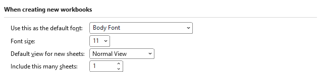
2. Click OK. Excel says the new font applies after a restart, so click OK again, then close and reopen Excel.

Fix #2: Save a Default Workbook Template (Book.xltx)

For styles, column widths, headers and footers, sheet counts, and page setup, use a default workbook template. Here are the steps:

1. Set up a blank workbook with the formatting and layout you want every new workbook to use.

2. Press F12, choose Excel Template (*.xltx) in Save as type, and name the file Book.

3. Save it in your XLSTART folder: C:\Users\<your user name>\AppData\Roaming\Microsoft\Excel\XLSTART. Paste %appdata%\Microsoft\Excel\XLSTART into the Save As dialog’s address bar, press Enter, and click Save.

4. Restart Excel. New workbooks you create with Ctrl+N now start from that template. File > New > Blank workbook and the Start screen’s Blank workbook still use Excel’s built-in defaults.

To control new worksheets you insert, save a template named Sheet.xltx in the same folder.

To return new workbooks to Excel’s defaults, delete Book.xltx from that folder.

Additional Notes About Excel Not Saving Formatting

• If one file loses formatting on every save, it may be damaged. Go to File > Open > Browse, select it, click the arrow beside Open, and choose Open and Repair.
• To check whether an add-in or a startup macro (such as your Personal Macro Workbook) is resetting formatting, start Excel in Safe Mode. Hold Ctrl while you start Excel and click Yes, or run excel /safe from the Run box (Win+R).
• If the formatting buttons are grayed out and you’re not editing a cell, the sheet is probably protected. Go to Review > Unprotect Sheet (you’ll need the password if one was set).

Frequently Asked Questions

Here are a few related questions about missing formatting, CSV files, and workbook colors.

Why does my CSV still look formatted right after I save it?

Excel keeps showing what’s in memory until you close the file.

The CSV on disk only has the text, so the formatting is gone when you reopen it.

How do I stop the possible data loss warning when saving a CSV in Excel?

Go to File > Options > Save and uncheck <strong>Show data loss warning when editing comma delimited files (*.csv)</strong>.

This only hides the warning. A CSV still won’t keep your formatting.

Why does Excel remove leading zeros when I open a CSV file?

Excel reads a value such as 02134 as the number 2134 when it opens the CSV. The leading zero disappears during that conversion.

To keep it, import the CSV through Data > From Text/CSV and click Transform Data.

Click the type icon in the ZIP Code column header, choose Text, and click Replace current when Excel asks. Then click Close & Load.

In Microsoft 365, you can also go to File > Options > Data and find Automatic Data Conversion.

Uncheck Remove leading zeros and convert to a number, then reopen the CSV. This setting applies when opening .csv and .txt files.

Alternatively, keep the data in .xlsx with a 00000 number format or Text format for the ZIP codes.

Why do my colors change when I copy cells to another workbook?

Theme colors follow the workbook’s theme. When you paste into a workbook with a different theme, the same theme color slot can display a different color.

Use the same theme in both workbooks, or choose a standard or custom color instead of a theme color.

Conclusion

I’d check the file type first, especially if you’re saving as CSV, then look at refresh settings if widths change after an update.

The other fixes cover specific cases, from read-only copies to workbook defaults.

If you’re not sure where to start, check whether the file is .xlsx.

Other Excel articles you may also like:

• Excel Dates Not Formatting – How to Fix?
• How to Copy and Paste in Excel Without Changing the Format?
• Pivot Table Not Refreshing – How to Fix?
• Why is Excel so Slow? How to Fix Slow Excel Files!