How to Convert Text into a Formula in Excel

If your formulas show up as text like =C2*D2 instead of a result, you need a way to make Excel treat that text as a real formula and calculate it.

Excel only calculates a formula at the moment it’s entered in a cell. Text that just looks like a formula stays text, even after you change the cell format, until something makes Excel enter it again.

How you fix it depends on what the text looks like. If it already starts with an equal sign, a quick re-entry trick does the job.

If it’s only the math part, like 12*14, Excel needs more help, because no regular worksheet function calculates a text string.

In this article, I’ll show you five ways to convert text into formulas, using Find and Replace, Text to Columns, an old function called EVALUATE, and a short VBA function.

Convert Text Formulas That Start With an Equal Sign

These two methods work when your cells already hold complete formulas as text, like =C2*D2. This usually happens with imported data or with a column that was formatted as Text before the formulas went in.

Method #1: Using Find and Replace (Recommended)

Find and Replace is the fastest way to fix a whole column of text formulas. Replacing the equal sign with another equal sign sounds pointless, but it makes Excel enter every cell again, and that’s when it spots the formula.

Below I have a dataset of office supply orders. The Total column should show each order’s total, but it shows formulas like =C2*D2 as plain text.

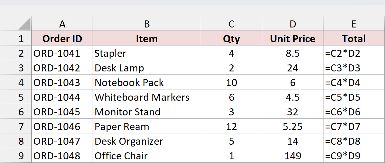
Here are the steps to convert this text into formulas:

1. Select the cells that have the text formulas (E2:E9 in this example).

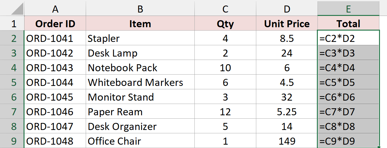
2. Press Ctrl + H to open the Find and Replace dialog box. Type = in the Find what field and = in the Replace with field.

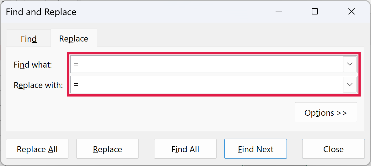
3. Click Replace All, then close the dialog box.

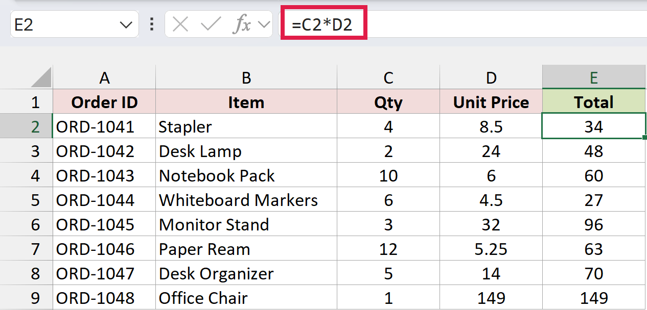
Excel calculates every cell, and the Total column now shows the order totals.

Find and Replace does skip cells that have an apostrophe in front of the formula (‘=C2*D2). Method #2 converts those too.

Note: If the cells were formatted as Text, they keep that format after the conversion. Edit one of them later and Excel turns it back into text. To avoid that, change the format of the column to General (Home tab, Number Format drop-down).

Method #2: Using Text to Columns

Text to Columns is built for splitting data, but it also enters each cell again when it runs. That makes it a handy fix, and unlike Find and Replace, it also converts formulas that have an apostrophe in front.

Below I have the same office supply orders, where the Total column has formulas stored as text.

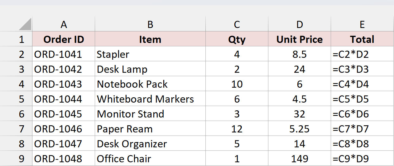
Here are the steps to convert the text formulas using Text to Columns:

1. Select the cells that have the text formulas (E2:E9).

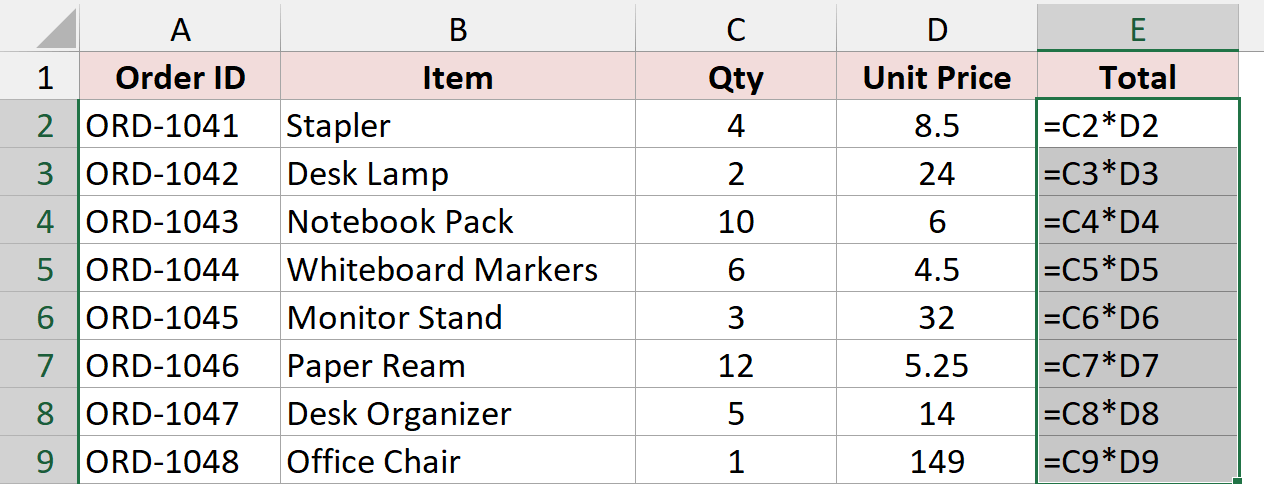
2. Click the Data tab, then click Text to Columns in the Data Tools group.

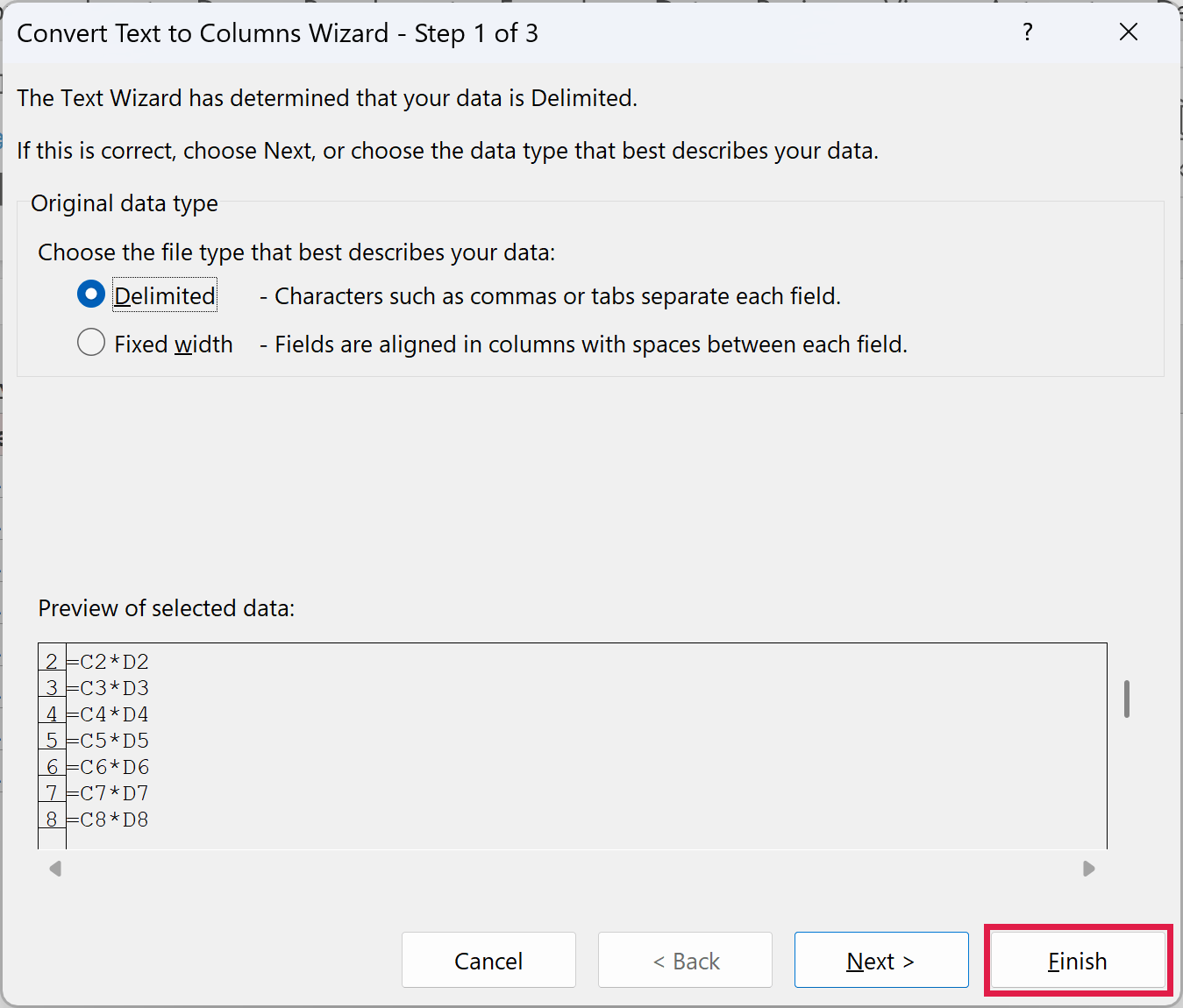
3. In the Convert Text to Columns Wizard, click Finish. You don’t need to change anything in the wizard.

Excel converts each text formula into a working formula and shows the totals.

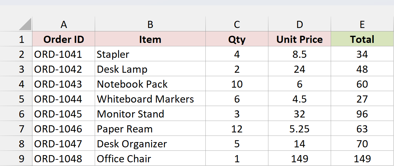
Text to Columns works on one column at a time. If your text formulas sit in several columns, run it on each column separately.

Note: Text to Columns remembers the delimiter you used last. If your formulas have commas or spaces in them, click Next in the wizard and clear every delimiter checkbox before you click Finish, or Excel may split the formula across columns.

Convert Text Expressions Without an Equal Sign

Sometimes the text is only the math part, like 12*14, with no equal sign in front. You see this a lot when measurements or quick calculations get typed in as notes. These three methods turn that kind of text into a result.

Method #3: Adding an Equal Sign With a Formula

If your expressions don’t start with an equal sign, you can add one with a formula and then use the Find and Replace trick from Method #1. You end up with regular formulas and no helper column.

Below I have a list of rooms with their floor measurements typed as text in column B. I want the area of each room in square feet.

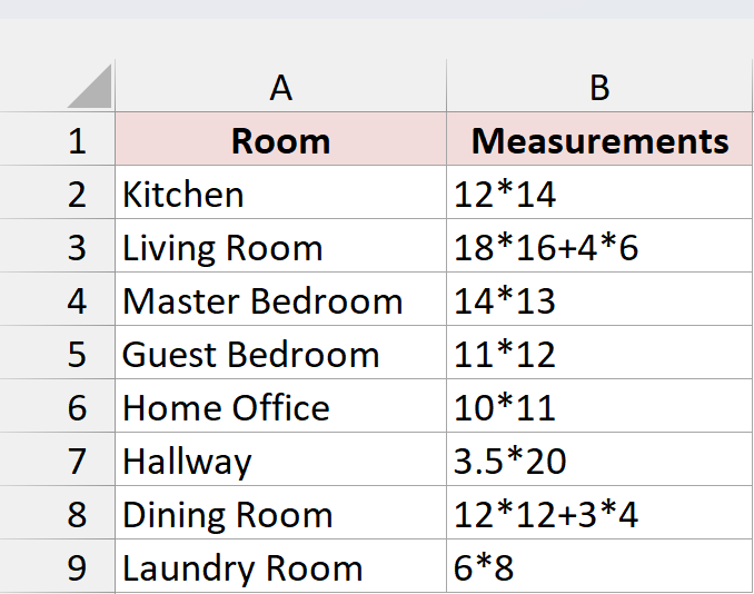
First, enter this formula in cell C2:

="="&B2:B9

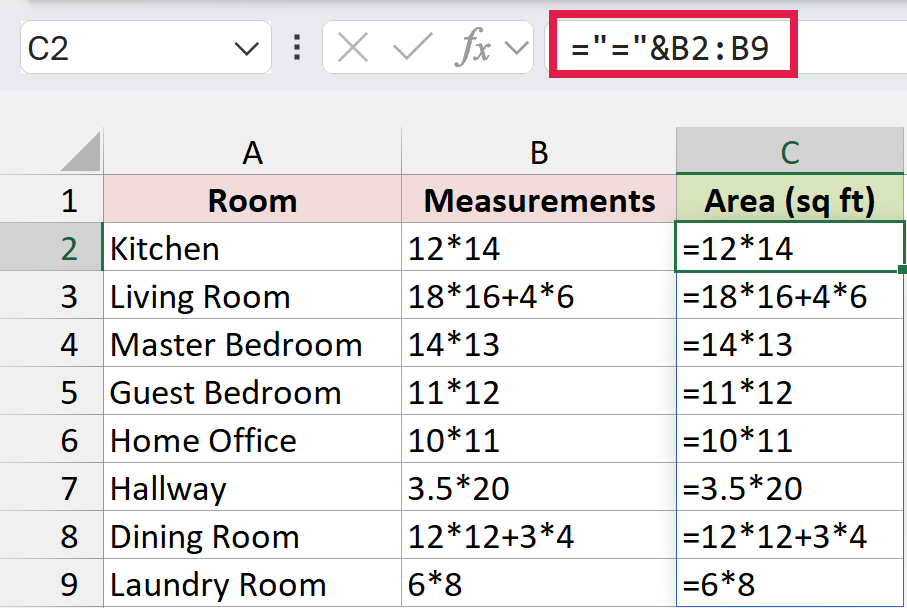
The formula joins an equal sign to the front of each measurement, so C2 shows =12*14. It spills down the column automatically, but the results are still text, not formulas. In Excel 2019 or older, enter =”=”&B2 in C2 instead and copy it down.

Here are the steps to turn this text into working formulas:

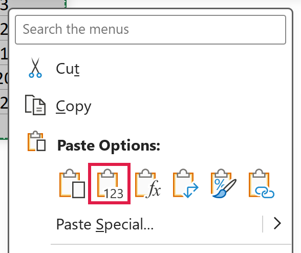
1. Select C2:C9 and press Ctrl + C to copy it. Then right-click the selection and click the Values icon under Paste Options.

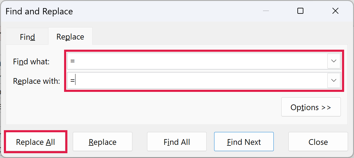
2. With C2:C9 still selected, press Ctrl + H. Type = in both the Find what and Replace with fields, then click Replace All and close the dialog box.

Column C now holds real formulas like =12*14, and each cell shows the area of the room.

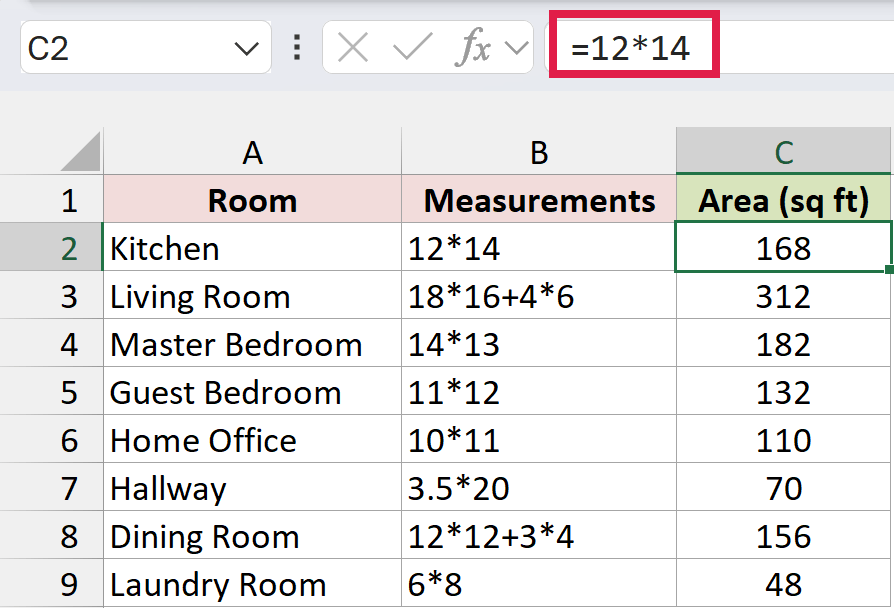
Note: The new formulas don’t look at column B anymore. If you change a measurement, the area won’t update. Use Method #4 or Method #5 if you need live results.

Method #4: Using EVALUATE in a Named Formula

Excel has an old function called EVALUATE that calculates a text expression. You can’t type it into a cell, though, because Excel rejects it there. It only works inside a defined name.

The upside is that the results stay live. Change a measurement, and the area updates right away.

Below I have the same list of rooms, with the measurements typed as text in column B.

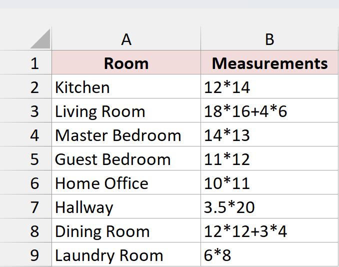
Here are the steps to calculate the text with EVALUATE:

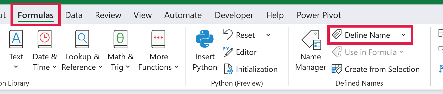
1. Select cell C2, then click the Formulas tab and click Define Name.

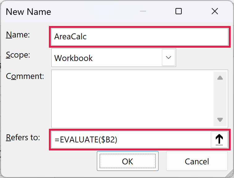
2. In the New Name dialog box, type AreaCalc in the Name field and =EVALUATE($B2) in the Refers to field, then click OK.

3. In cell C2, enter =AreaCalc and copy it down to C9.

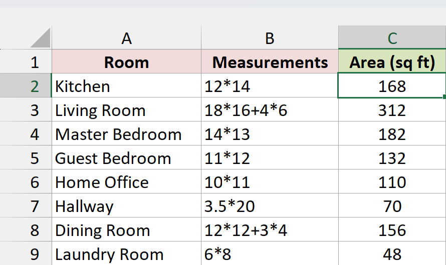
Each cell in column C now shows the area for its room.

How does this work?

The name AreaCalc runs EVALUATE on column B of the same row. The $ locks the column, but the row stays relative to C2, the cell you selected when you created the name.

So C3 reads B3, C4 reads B4, and so on. Excel also adds the sheet name to the reference on its own.

Because the name works one row at a time, it doesn’t spill. That’s why you copy it down instead.

Note: EVALUATE counts as macro content, so save the file as an Excel Macro-Enabled Workbook (.xlsm). A regular .xlsx file can’t hold it.

Method #5: Using a VBA Custom Function

If you’d rather have a function you can type into any cell, a few lines of VBA create one. After that, =EvalText(B2:B9) works just like a built-in function and spills the results down the column.

Below I have the list of rooms again, with the measurements typed as text in column B.

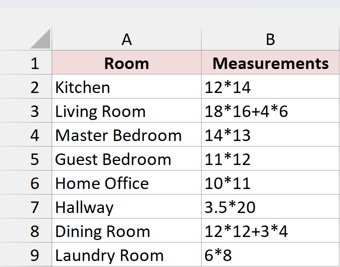
Here is the VBA code:

Function EvalText(expr As Variant) As Variant
    Dim ws As Worksheet, v As Variant, out() As Variant, r As Long, c As Long
    Application.Volatile
    Set ws = Application.Caller.Parent
    If TypeName(expr) = "Range" Then v = expr.Value Else v = expr
    If Not IsArray(v) Then
        EvalText = ws.Evaluate(CStr(v))
        Exit Function
    End If
    ReDim out(1 To UBound(v, 1), 1 To UBound(v, 2))
    For r = 1 To UBound(v, 1)
        For c = 1 To UBound(v, 2)
            If Len(v(r, c)) > 0 Then out(r, c) = ws.Evaluate(CStr(v(r, c))) Else out(r, c) = ""
        Next c
    Next r
    EvalText = out
End Function

Function EvalText(expr As Variant) As Variant
    Dim ws As Worksheet, v As Variant, out() As Variant, r As Long, c As Long
    Application.Volatile
    Set ws = Application.Caller.Parent
    If TypeName(expr) = "Range" Then v = expr.Value Else v = expr
    If Not IsArray(v) Then
        EvalText = ws.Evaluate(CStr(v))
        Exit Function
    End If
    ReDim out(1 To UBound(v, 1), 1 To UBound(v, 2))
    For r = 1 To UBound(v, 1)
        For c = 1 To UBound(v, 2)
            If Len(v(r, c)) > 0 Then out(r, c) = ws.Evaluate(CStr(v(r, c))) Else out(r, c) = ""
        Next c
    Next r
    EvalText = out
End Function

Here are the steps to use this function:

1. Save your workbook as an Excel Macro-Enabled Workbook (.xlsm). If you’re using the example file, click Enable Editing first if Protected View shows, and use the Text Expressions sheet.
2. Press Alt + F11 to open the VB Editor. On a Mac, go to Tools > Macro > Visual Basic Editor.
3. Click Insert, then Module.
4. Paste the code above into the module and close the VB Editor.
5. In cell C2, enter =EvalText(B2:B9). The results spill down to C9 automatically.

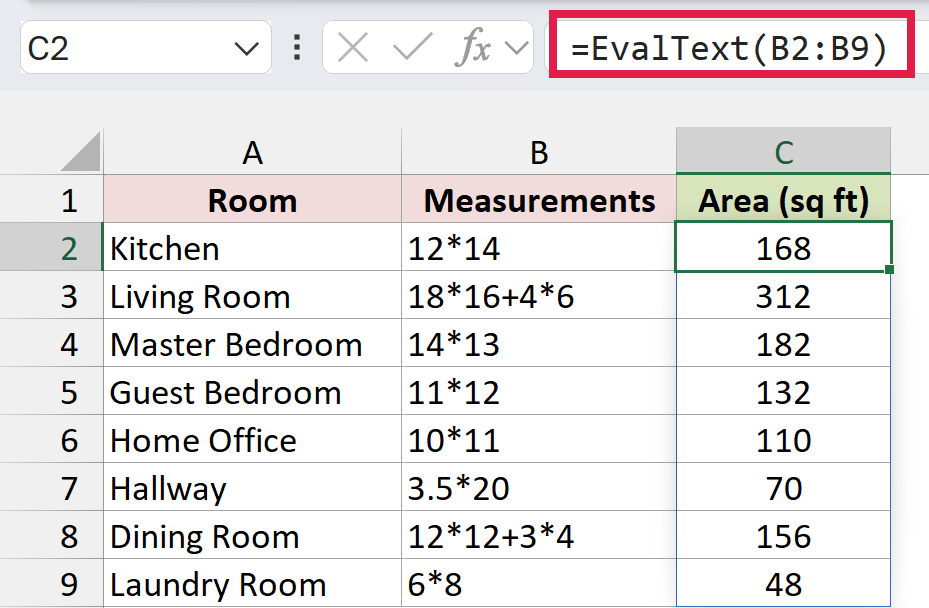
How does this code work?

EvalText takes each text value in the range and hands it to Excel’s own Evaluate method, which calculates it the same way a cell formula would. It returns the answers as a list, so Excel spills them into C2:C9.

You can also give it a single cell. =EvalText(B2) returns 168. In Excel 2019 or older, results don’t spill, so use =EvalText(B2) in C2 and copy it down.

Application.Caller.Parent makes it run on the sheet where the formula sits, so cell references in the text point to the right place. Application.Volatile makes it recalculate whenever the sheet does, which matters when the text refers to other cells, like SUM(C2:C4).

Additional Notes About Converting Text into Formulas in Excel

• If every formula on the sheet shows as text, check the Show Formulas setting first. Press Ctrl + the grave accent key (the one above Tab) to switch it off. When Excel is showing formulas instead of results, it’s often a display setting, not a text problem.
• EVALUATE and the VBA function both return #VALUE! when the text is longer than 255 characters, so keep each expression short.
• Methods #1 to #3 leave you with ordinary formulas, so the file stays a normal .xlsx. Methods #4 and #5 need a macro-enabled file, and VBA doesn’t run in Excel for the web.

Frequently Asked Questions

Here are a few questions people often ask about turning text into formulas.

Can the INDIRECT function convert text into a formula?

No. INDIRECT turns text into a cell reference, so “B2” returns the value in B2. It can’t calculate an expression like 12*14.

Is there an EVAL function in Excel 365?

No. Excel doesn’t have a regular worksheet function that calculates text. EVALUATE only works inside a defined name, which is why Method #4 uses one.

How do I turn a formula back into text?

Use the FORMULATEXT function. =FORMULATEXT(E2) returns the formula in E2 as text, while E2 keeps working.

Conclusion

In this article, I showed you five ways to convert text into formulas in Excel. If your text formulas already start with an equal sign, Find and Replace is the quickest one to try first.

I hope you found this article helpful.

Other Excel articles you may also like:

• How to Remove Formulas in Excel (and keep the data)
• Show Formulas (Instead of Formula Result) in Excel (Shortcut)
• How to Convert Text to Date in Excel?
• VALUE Function in Excel
• How to Add Double Quotes in an Excel Formula
• How To Hide Formulas In Excel Without Protecting the Sheet?