
The BITOR function in Excel returns a number whose bits are switched on wherever either input number has the matching bit switched on.
It’s useful for merging option codes because shared flags are included once. Unlike addition, BITOR doesn’t carry an already active flag into another bit.
In this article, I’ll show you how to merge code lists, switch flags on safely, and combine several codes without double-counting shared options.
BITOR Function Syntax in Excel
The BITOR function accepts two numbers and combines their active bits.
=BITOR(number1, number2)
- number1 (required) is the first nonnegative whole number containing the bits you want to combine.
- number2 (required) is the second nonnegative whole number containing the bits you want to combine.
BITOR accepts exactly two arguments. Both inputs can contain several flags, with each flag represented by a separate power of 2.
BITOR is available in Excel 2013 and later.
When to Use BITOR Function
- Merge two option, permission, or feature codes without counting shared flags twice.
- Switch a particular flag on while preserving every flag already present.
- Apply a new flag only to rows that meet a condition.
- Combine several code columns or a whole list into one code.
Example 1: Combine Two Numbers With BITOR
Let’s start by seeing what BITOR does at the bit level.
Below is the dataset. Columns A and B hold number pairs, while columns C through F will show the BITOR result and binary views.
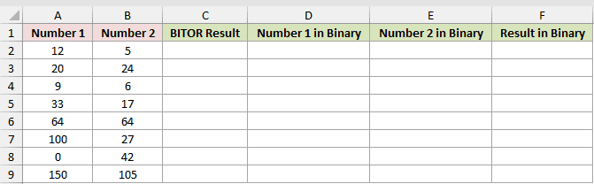
We want to combine each pair with one spilling BITOR formula.
Here is the BITOR formula:
=BITOR(A2:A9,B2:B9)
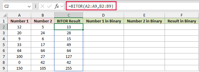
To make the bit pattern visible, here is the BASE formula:
=BASE(A2:C9,2,8)
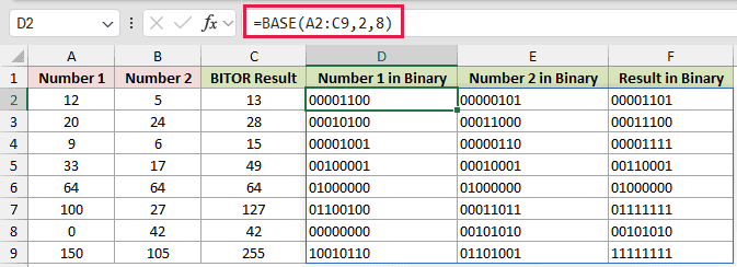
The first formula spills results down column C. BITOR keeps each bit that appears in either number, while shared bits remain switched on only once.
For the first pair, 12 and 5 return 13. The binary view shows 00001100 and 00000101 combining into 00001101.
The BASE formula spills an 8-digit binary view of all three number columns, which makes overlapping bits much easier to spot.
Pro Tip: These range formulas spill in Excel 2021, Excel 2024, and Microsoft 365. In Excel 2019 and earlier, enter a per-row version and fill it down.
Example 2: Merge Two Device Code Lists
Here’s a practical row-by-row merge.
Below is the dataset. It lists customers, installed-device codes, new-order codes, a device legend, and a result column for the combined code.
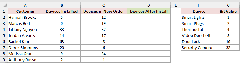
We want one formula to combine the installed and newly ordered devices for every customer.
Here is the formula:
=BITOR(B2:B9,C2:C9)
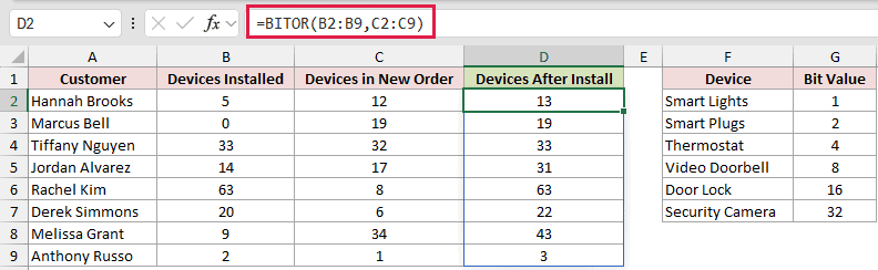
BITOR combines the two codes on each row. A device found in both lists still occupies one bit in the updated code.
Hannah Brooks has codes 5 and 12, which return 13. Tiffany Nguyen has codes 33 and 32, but her combined code remains 33.
Tiffany’s Security Camera flag was already active. BITOR preserves it without counting that device again.
Example 3: Turn On a Flag Safely
This example shows why adding a flag value can quietly break a code.
Below is the dataset. It lists attendee extras codes and the extras legend in columns F:G, with headers Extra and Bit Value.
The legend runs from Workshop Pass 1 through Printed Workbook 32.
It also includes a BITOR result column and an addition column that’s deliberately shown as the wrong method.
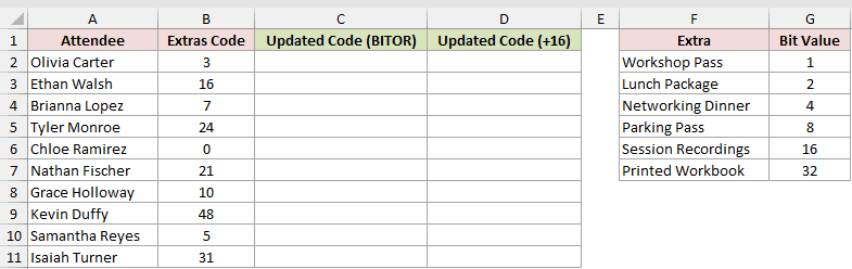
We want to switch on the Session Recordings flag for every attendee without disturbing existing extras.
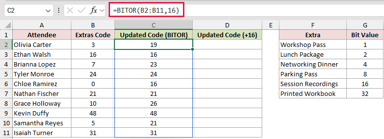
Here is the correct BITOR formula:
=BITOR(B2:B11,16)
This next formula is the mistake. It adds 16 instead of safely switching on the matching flag.
=B2:B11+16
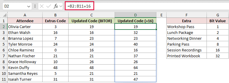
The BITOR formula leaves an existing Session Recordings flag unchanged. The mistaken addition carries that bit into the next position when it’s already on.
Ethan Walsh starts with 16. BITOR correctly returns 16, while the mistaken addition returns 32, meaning Printed Workbook only and losing his Session Recordings extra.
Kevin Duffy starts with 48. BITOR correctly keeps 48, while the mistaken addition returns 64, which matches no extra in the legend.
Pro Tip: BITOR only switches flags on. It never switches an existing flag off, even when the same flag appears in both inputs.
Example 4: Add a Flag Conditionally
Now let’s turn on a perk only for customers who qualify.
Below is the dataset. It contains annual spending, current perks codes, a perks legend, and an output column for each updated code.
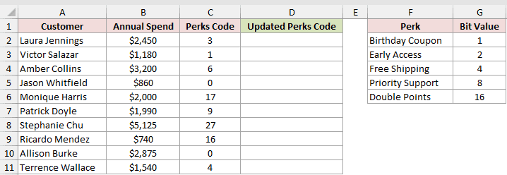
We want to add Free Shipping for customers whose annual spending is at least $2,000.
Here is the formula:
=BITOR(C2:C11,IF(B2:B11>=2000,4,0))
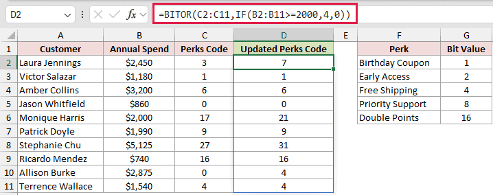
IF returns 4 for qualifying rows and 0 otherwise. OR with 0 leaves the current code unchanged.
Laura Jennings moves from code 3 to 7. Amber Collins stays at 6 because Free Shipping was already included in her code.
Monique Harris qualifies at exactly $2,000 and moves from 17 to 21. Terrence Wallace stays at 4 despite falling below the threshold.
BITOR can add the qualifying perk, but it doesn’t remove an existing perk from someone who no longer qualifies.
Example 5: Combine Three Option Codes
BITOR accepts two arguments, so a third source needs another BITOR call.
Below is the dataset. Each vehicle order has three option-code columns, a flag legend, and an All Options column for the merged code.
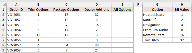
We want to merge all three option sources for every order.
Here is the nested formula:
=BITOR(BITOR(B2:B9,C2:C9),D2:D9)
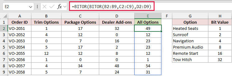
The inner BITOR combines the Trim and Package codes. The outer BITOR then merges that result with the Dealer Add-ons code.
VO-2051 combines 1, 17, and 32 into 49. That result represents Heated Seats, Remote Start, and Tow Hitch.
VO-2055 contains 12, 12, and 8, yet BITOR returns 12. Addition would return the wrong code, 32, because shared options were counted more than once.
In Microsoft 365 and Excel 2024, BYROW with REDUCE can scale this pattern across more code columns.
Use =BYROW(B2:D9,LAMBDA(r,REDUCE(0,r,LAMBDA(a,x,BITOR(a,x))))). It returns the same results as column E.
Example 6: Combine a Whole Code Column
Nesting becomes awkward when the codes run down a long list.
Below is the dataset. It lists department module codes, a module legend, and a labelled result cell for the combined company license code.
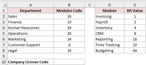
We want one company code containing every module used by any department.
Here is the formula:
=REDUCE(0,B2:B8,LAMBDA(combined,dept,BITOR(combined,dept)))
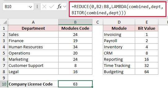
REDUCE starts with 0 and processes each department code. BITOR carries the combined flags forward until the list has been folded into one result.
The formula returns 63. It includes Invoicing, Payroll, Inventory, CRM, Reporting, and Time Tracking, while Budgeting remains unused.
SUM returns 145 for these same codes. That’s wrong because overlapping module flags are counted repeatedly.
Pro Tip: REDUCE and LAMBDA require Microsoft 365 or Excel 2024. Excel 2021 returns #NAME?, so use nested BITOR calls or a running helper column there.
Tips & Common Mistakes
- BITOR works with nonnegative whole numbers from 0 through 281474976710655. Decimals, negative numbers, and values above that limit return
#NUM!. - Numbers stored as text are converted. TRUE is treated as 1, a blank cell as 0, and other text such as “abc” returns
#VALUE!. - BITOR switches flags on. Use BITAND when you need to test or clear bits, and BITXOR when you need to toggle them.
- A blocked spill range returns
#SPILL!. Clear the cells below and beside the formula so Excel can place the complete result. - Plain addition is unsafe when codes share a flag. The shared value is counted again and can carry into another bit.
- BITOR accepts exactly two arguments. Nest it for a few codes, or use REDUCE when you need to combine a column.
BITOR is safest when each flag is a separate power of 2. Overlapping options then stay in one bit, even after several codes are merged.
Use addition only when you’ve proved the flag is off.
Related Excel Functions / Articles:
