
The GAUSS function in Excel returns the signed area between the mean and a z-score on the standard normal curve.
A z-score tells you how far a value sits above or below the mean in standard deviations. GAUSS translates that distance into an area under the curve.
A negative z-score returns a negative area, so keep the sign in mind before reporting the result as a share.
I’ll show you how to interpret negative results and estimate the share of measurements within a tolerance band.
GAUSS Function Syntax in Excel
GAUSS takes a z-score as its argument:
=GAUSS(z)
- z (required) is the standardized value you want to evaluate. It can be a number, a cell reference, or a range of z-scores.
Positive inputs return positive areas, and negative inputs return negative areas. At the mean, GAUSS returns zero.
When to Use GAUSS Function
- Find the signed area between the mean and a particular z-score.
- Convert measurements into z-scores and assess their position relative to a target mean.
- Estimate the share of normally distributed measurements within a symmetric tolerance band.
- Calculate the chance of exceeding a target or landing between specified limits under a normal model.
Example 1: Compare GAUSS With NORM.S.DIST
An area measured from the mean differs from a cumulative probability.
Below is the dataset. Column A holds z-scores; column B will hold GAUSS results, column C the NORM.S.DIST comparison, and column D a difference check.
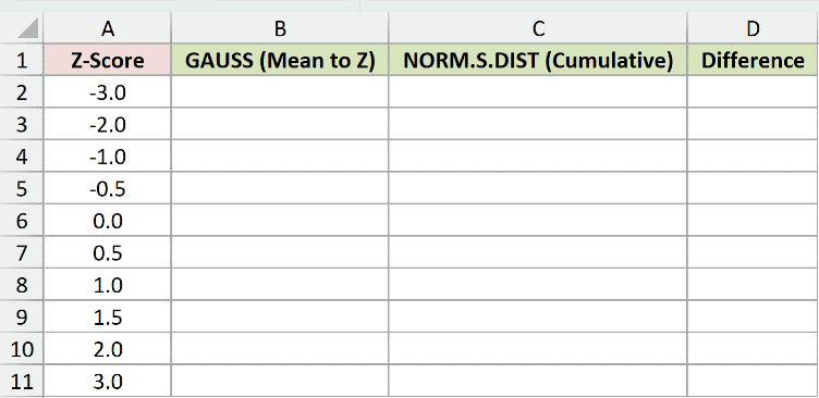
We want the signed area for each z-score, then a comparison showing how it relates to the cumulative probability.
Enter this formula in B2:
=GAUSS(A2:A11)
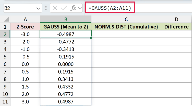
The formula spills into B2:B11. At a z-score of -1.0, it returns -0.3413; at 1.0, it returns 0.3413.
Those matching magnitudes reflect the curve’s symmetry. The negative sign identifies the side below the mean; the magnitude gives the proportion between that input and the mean.
Range formulas spill in Excel 2021, Excel 2024, and Microsoft 365. In Excel 2019 and earlier, use a single-cell reference and fill the per-row formula down.
For the cumulative comparison, enter this formula in C2:
=NORM.S.DIST(A2:A11,TRUE)
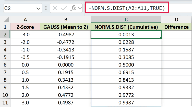
The comparison spills into C2:C11. NORM.S.DIST with TRUE measures the entire area to the left of each z-score, rather than starting at the mean.
For -1.0, the cumulative comparison returns 0.1587. For 1.0, it returns 0.8413.
Now enter the difference check in D2:
=C2:C11-B2:B11
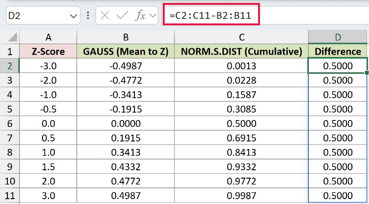
Every row of this check displays 0.5000. GAUSS is the cumulative standard normal probability minus 0.5, including when the z-score is negative.
Example 2: Convert Bolt Lengths Into Signed Areas
Real measurements need converting before GAUSS can use them.
Below is the dataset. Columns A and B list bolts and lengths; E:F holds the target and standard deviation, and column C will hold signed areas.
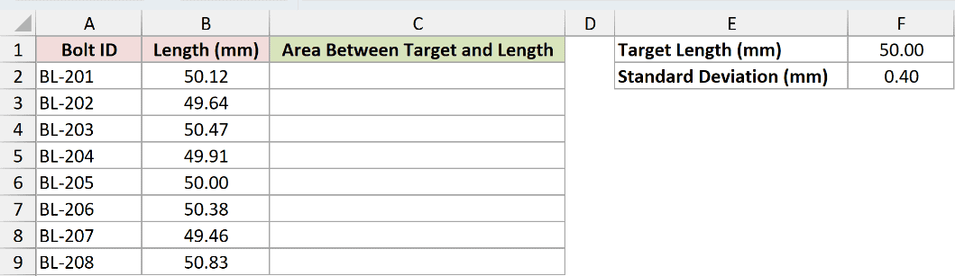
We want the signed area between the target mean and each measured length, assuming bolt lengths follow a normal distribution centered on that target.
Enter this formula in C2:
=GAUSS(STANDARDIZE(B2:B9,F1,F2))
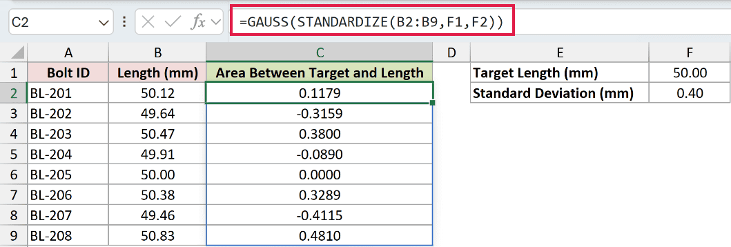
STANDARDIZE subtracts the target in F1 from each length, then divides by the standard deviation in F2. GAUSS evaluates those z-scores and spills into C2:C9.
The input card holds a target of 50.00 mm and a standard deviation of 0.40 mm. These are typed model inputs.
BL-201 measures 50.12 mm and returns 0.1179. BL-202 measures 49.64 mm and returns -0.3159, because it’s below the target mean.
BL-205 is exactly 50.00 mm, so its signed area is 0.0000. There’s no distance between that measurement and the target.
Pro Tip: Use ABS on a GAUSS result for the area between the mean and measurement regardless of side. Keep the sign to distinguish below-target from above-target measurements.
Example 3: Estimate Bolts Within a Tolerance
A band around the target mean lets us estimate the share of bolts within tolerance.
Below is the dataset. Column A lists tolerance distances, F1 holds the standard deviation, and columns B and C will hold standardized distances and within-tolerance shares.
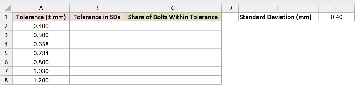
We want the expected share of bolts within each symmetric tolerance, assuming the normal process remains centered on its target.
First, convert the tolerance distances to standard deviations in B2:
=A2:A8/F1
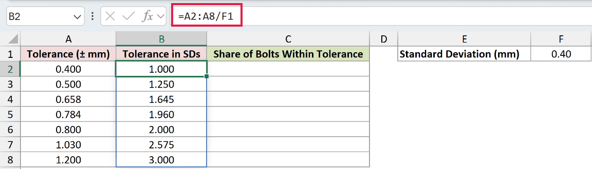
This spills into B2:B8. A tolerance of 0.400 mm becomes 1.000 standard deviations; 0.784 mm becomes 1.960.
Next, calculate the central share in C2:
=2*GAUSS(B2:B8)
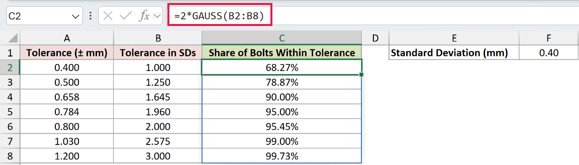
GAUSS measures the area from the mean to the positive tolerance limit. Multiplying by 2 includes the matching area below the mean.
The results spill into C2:C8. The expected share within ±0.400 mm is 68.27%, while ±0.784 mm covers 95.00%.
Widening the band to ±0.800 mm returns 95.45%. At ±1.200 mm, the share is 99.73%.
These shares come from the assumed normal model. Counting the measured bolts in Example 2 would describe that sample instead.
A process that drifts away from its target needs different limits.
Example 4: Find Chances Above and Below Targets
A coffee shop can use the same signed area to estimate either side of a sales target.
Below is the dataset. Column A lists daily cup targets; E:F holds the mean and standard deviation, with columns B and C reserved for above-target and below-target shares.

We want the approximate share of days above and below each target, using a normal model for daily cup sales.
Enter the above-target formula in B2:
=0.5-GAUSS((A2:A6-F1)/F2)
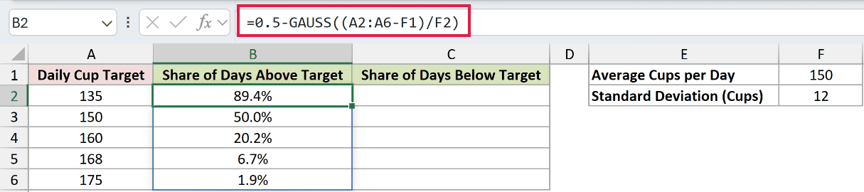
The arithmetic inside GAUSS standardizes each target using the mean of 150 cups and standard deviation of 12 cups. The results spill into B2:B6.
Subtracting the signed area from 0.5 leaves the right tail. The estimated share above 135 cups is 89.4%; above 175, it’s 1.9%.
The lower target produces a negative GAUSS result. Subtracting that negative area correctly increases the above-target share.
For the below-target share, enter this formula in C2:
=0.5+GAUSS((A2:A6-F1)/F2)
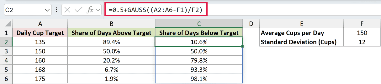
Adding the signed area to 0.5 returns the left tail and spills into C2:C6.
The estimated share below 135 cups is 10.6%, while below 175 it’s 98.1%. At the mean of 150, both columns display 50.0%.
Example 5: Calculate Chances Between Sales Limits
The limits don’t have to sit equally far from the mean.
Below is the dataset. Columns A:E contain locations, average sales, standard deviations, and lower and upper limits. Column F will hold the chance of landing inside each range.

We want the probability of daily sales falling between each location’s limits, assuming its sales follow a normal distribution.
Enter this formula in F2:
=GAUSS((E2:E6-B2:B6)/C2:C6)-GAUSS((D2:D6-B2:B6)/C2:C6)
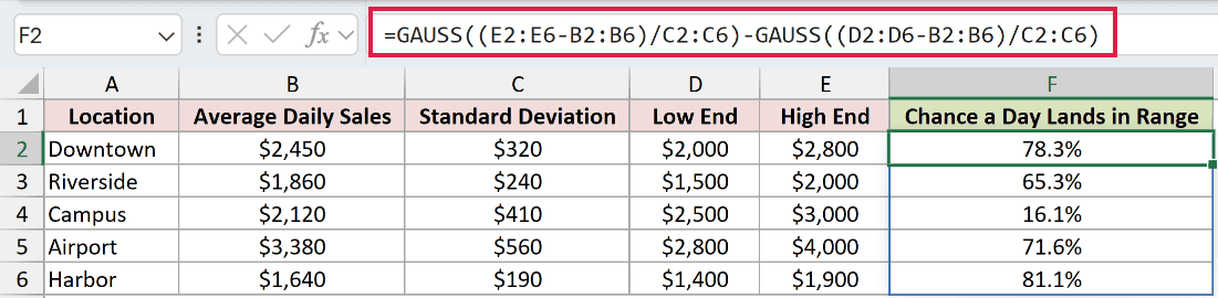
How this formula works:
- The first GAUSS calculation standardizes each upper limit using that location’s mean and standard deviation.
- The second GAUSS calculation does the same for the lower limit.
- Subtracting the lower signed area from the upper signed area leaves the probability between the limits. The results spill into
F2:F6.
Downtown’s range of $2,000 to $2,800 returns 78.3%. Harbor’s range of $1,400 to $1,900 returns 81.1%.
Both Campus limits, $2,500 and $3,000, sit above its $2,120 mean. The probability between them is 16.1%.
You don’t need a separate formula for ranges that cross the mean. The signs handle that automatically, provided the upper limit stays above the lower limit.
Tips & Common Mistakes
- GAUSS needs a z-score. Standardize raw lengths, sales, or other measurements before passing them to GAUSS. Otherwise, Excel interprets the raw number as a distance in standard deviations.
- NORM.DIST accepts raw measurements. With NORM.DIST,
=NORM.DIST(x,mean,sd,TRUE)-0.5returns the signed area without a separate standardization step. - Negative results are expected. GAUSS returns a signed area. Use ABS when you need its magnitude, but preserve the sign when calculating tails or subtracting interval endpoints.
- Check blank inputs. In testing, a truly blank cell returned 0. A missing measurement can therefore look like a value exactly at the mean.
- Text behavior depends on the content. Numeric text converts, while nonnumeric text returns
#VALUE!. Check imported z-scores before using them. - GAUSS is available in Excel 2013 and later. The range-based examples require a version that supports spilling, as explained in Example 1.
- Keep spill destinations clear. Existing content in the output area can cause
#SPILL!. An@before a range-based function forces implicit intersection instead of the intended spill. - Choose the area your question needs. NORM.S.DIST is more direct for a cumulative probability. GAUSS is convenient for areas measured from the mean and symmetric tolerance bands.
- A two-tailed normal p-value uses the area outside the central band. Double the GAUSS area for the absolute z-score, then subtract it from the whole distribution.
Try changing a tolerance in Example 3 to see how the expected share responds.
Keep the standard deviation tied to the process you’re modeling.
Related Excel Functions / Articles:
