
The ISLOGICAL function in Excel checks whether a value is a real logical TRUE or FALSE. It returns TRUE for either logical value and FALSE for anything else.
That distinction matters when imported data mixes real logicals with text that looks identical. A cell displaying TRUE can still contain text, so appearance alone doesn’t tell you its type.
I’ll show you how ISLOGICAL identifies valid flags, spots imported TRUE/FALSE text that needs fixing, and checks which entries belong in a count or review list.
ISLOGICAL Function Syntax in Excel
ISLOGICAL takes the value you want to check:
=ISLOGICAL(value)
- value (required) is the value, cell reference, or expression to test. You can also pass a range to check its cells individually.
The FALSE function returns the logical value FALSE, which passes ISLOGICAL. ISLOGICAL checks the value’s type, not whether a condition was met.
When to Use ISLOGICAL Function
- Check whether imported flags contain real logical values or text lookalikes.
- Inspect formulas that should return logical flags but instead return labels or numbers.
- Count valid TRUE/FALSE entries in a checklist, including unfinished items marked FALSE.
- Build a review list of records whose flags need correcting.
Example 1: Check Survey Responses for Logical Values
Let’s start with a survey export containing different kinds of responses.
Below is the dataset. Column A lists survey questions, column B holds responses, and column C is set up for the Is Logical? results.
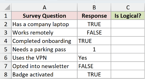
We want to identify which responses are stored as real logical values.
Enter this formula in C2:
=ISLOGICAL(B2:B8)
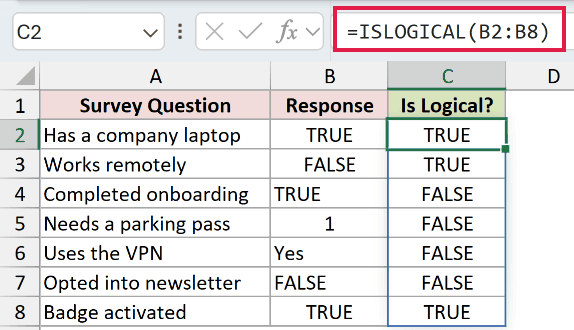
The formula spills into C2:C8, checking each response separately. The results are TRUE, TRUE, FALSE, FALSE, FALSE, FALSE, and TRUE.
This spill works in Excel 2021, Excel 2024, and Microsoft 365. In Excel 2019 and earlier, check each response with a single-cell reference and fill down.
The company-laptop response in B2 contains real TRUE, while the remote-work response in B3 contains real FALSE. Both pass, so C2 and C3 return TRUE.
The onboarding response in B4 displays TRUE but contains text. Its check returns FALSE, as does the text FALSE in B7.
The number 1 in B5 and the label Yes in B6 also return FALSE. Neither is a logical value, even if someone intended it as an affirmative response.
Pro Tip: Type an apostrophe before TRUE to store it as text. Entering TRUE in a General cell can create a real logical value.
Example 2: Test Flags Returned by Formulas
A formula can return a logical value, text, or a number, depending on how you write it.
Below is the dataset. Column A describes each flag formula, column B contains the calculated flags being tested, and column C will hold the type checks.
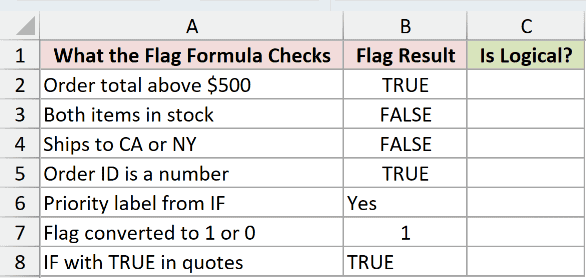
We want to find which existing flag formulas actually return logical values.
Enter this formula in C2:
=ISLOGICAL(B2:B8)
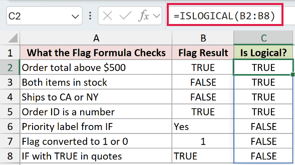
The formula spills into C2:C8. Here’s what the existing formulas in column B show:
B2contains=720>500, which returns TRUE. The type check inC2returns TRUE.B3contains=AND(12>0,0>0). AND checks whether all conditions are true. Here it returns logical FALSE, so ISLOGICAL inC3returns TRUE.B4contains=OR("TX"="CA","TX"="NY"). OR checks whether any condition is true. Here it returns logical FALSE, so ISLOGICAL inC4returns TRUE.B5contains=ISNUMBER(10452). ISNUMBER checks whether a value is a number. Here it returns logical TRUE, so ISLOGICAL inC5returns TRUE.B6contains=IF(720>500,"Yes","No"). IF chooses between two results based on a condition. Here it returns text Yes, so ISLOGICAL inC6returns FALSE.B7contains=--(720>500), which returns the number 1. The type check inC7returns FALSE.B8contains=IF(720>500,"TRUE","FALSE"), which returns the text TRUE. The type check inC8returns FALSE.
The quoted TRUE/FALSE outputs in B8 are the mistake if your goal is a logical flag. The comparison itself is logical, but IF returns the quoted text you supplied.
Similarly, the double minus in B7 converts the comparison’s logical result into a number. That’s useful for arithmetic, but the result no longer passes ISLOGICAL.
Example 3: Fix Imported TRUE and FALSE Text
Now let’s use the check to clean up an imported customer list.
Below is the dataset. Columns A and B contain customer accounts and imported active flags. Columns C and D are prepared for check labels and corrected flags.
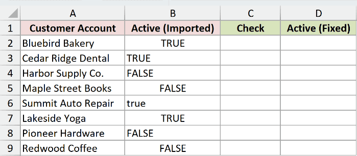
We want to flag the text entries, then convert them while preserving the existing logical values.
First, enter this formula in C2:
=IF(ISLOGICAL(B2:B9),"OK","Text - fix")
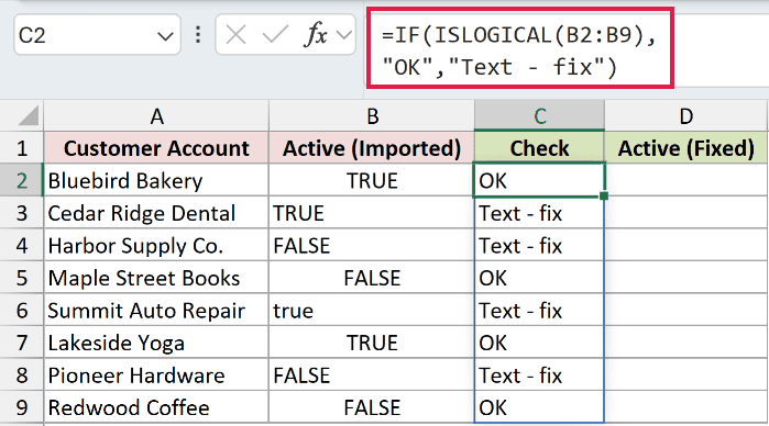
The labels spill into C2:C9. Bluebird Bakery returns OK, while Cedar Ridge Dental and Harbor Supply Co. return Text – fix.
The Text – fix label fits this dataset because all its non-logical entries are text flags.
Next, enter the conversion formula in D2:
=IF(ISLOGICAL(B2:B9),B2:B9,B2:B9="TRUE")
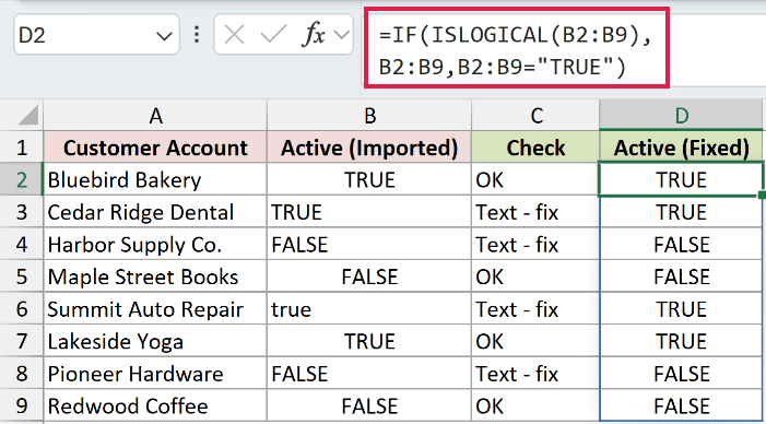
The corrected flags spill into D2:D9: TRUE, TRUE, FALSE, FALSE, TRUE, TRUE, FALSE, and FALSE.
How this formula works:
- ISLOGICAL checks each imported flag.
- When the flag is already logical, IF keeps its original value.
- Otherwise, the comparison against the text TRUE produces a real logical result.
Cedar Ridge Dental’s text TRUE becomes logical TRUE. Harbor Supply Co.’s text FALSE becomes logical FALSE.
The lowercase true for Summit Auto Repair also becomes TRUE. The text comparison here isn’t case-sensitive.
Pro Tip: Use this conversion only when the text entries are known TRUE/FALSE flags. An unexpected label would fail the comparison and become FALSE, hiding an entry that needs review.
Example 4: Count Logical Values in a Checklist
Below is the dataset. Columns A and B hold office-move tasks and completion flags. The Measure and Count card in columns D and E will summarize them.
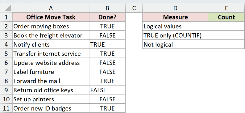
We want to count valid logical entries, compare that with completed tasks, and count the entries needing correction.
For the logical-value count, enter this formula in E2:
=SUM(--ISLOGICAL(B2:B11))
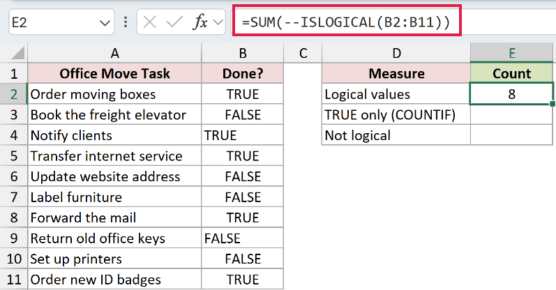
The result is 8.
ISLOGICAL tests every cell, and the double minus converts TRUE to 1 and FALSE to 0. SUM adds those numbers to count the logical entries.
COUNTIF counts cells that match a condition. In E3, it counts only real TRUE entries, letting us compare completed tasks with the ISLOGICAL count:
=COUNTIF(B2:B11,TRUE)
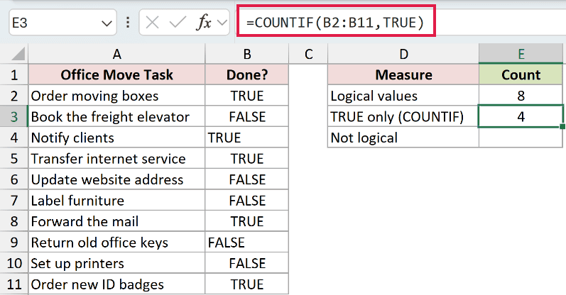
This comparison returns 4. It counts completed tasks marked with real TRUE, leaving out real FALSE and the text TRUE entry for Notify clients.
COUNTIF counts completed tasks; the ISLOGICAL count includes both real TRUE and real FALSE flags.
To count the non-logical entries, enter this formula in E4:
=SUM(--NOT(ISLOGICAL(B2:B11)))
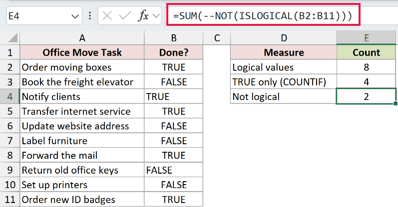
The result is 2. Notify clients and Return old office keys contain text flags and need correction.
NOT changes TRUE to FALSE and FALSE to TRUE. Here it reverses the ISLOGICAL results so the double minus and SUM count entries that failed the check.
Example 5: Filter Entries That Need Fixing
A separate review list saves you from searching through the source column for each bad flag.
Below is the dataset. Columns A and B list employees and benefits-enrollment entries. Columns D and E are prepared for employee names and entries to fix.
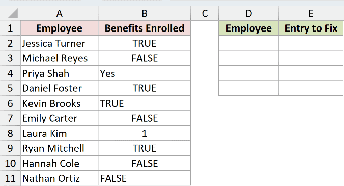
We want to extract the employees whose enrollment entries aren’t real logical values.
Enter this formula in D2:
=FILTER(A2:B11,NOT(ISLOGICAL(B2:B11)),"All clean")
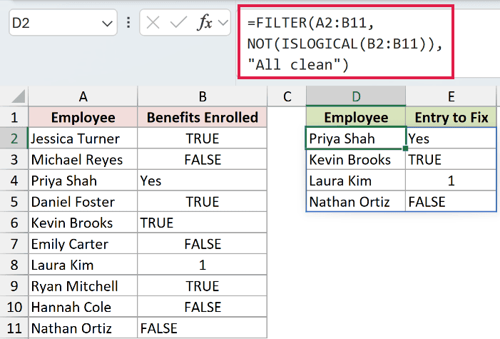
The result spills into D2:E5, showing these entries:
- Priya Shah: Yes.
- Kevin Brooks: TRUE stored as text.
- Laura Kim: 1.
- Nathan Ortiz: FALSE stored as text.
ISLOGICAL checks the enrollment column, and NOT reverses the results so failed checks become TRUE.
FILTER returns rows that meet a condition. Here it uses those TRUE results to list each employee whose flag failed ISLOGICAL, alongside the original entry.
Employees with real FALSE flags stay out of the review list. Their flags have the expected type, even though they aren’t enrolled.
The final argument provides the message All clean when no entries fail the check. FILTER requires Excel 2021 or later, including Microsoft 365.
Tips & Common Mistakes
- FALSE is a valid logical value, so it passes ISLOGICAL.
- Quoted TRUE/FALSE outputs from IF are text. Check the formula producing the flag when a logical-looking value fails.
- A blank cell or an error such as
#N/Areturns FALSE from ISLOGICAL. A failed check doesn’t tell you which non-logical type you have. - Keep the destination cells clear, and edit a spilling formula at its starting cell.
- Check unfamiliar labels before converting them. The import conversion assumes text flags have known meanings. Use the review-list approach when the input can include other labels or numbers.
- The TYPE function identifies a value’s type with a number, returning 4 for logical values. The older equivalent test
TYPE(value)=4checks for logicals, like ISLOGICAL.
ISLOGICAL checks both typed values and formula results for real TRUE/FALSE values.
You can use it to fix known text flags, count logical entries, and filter records that need review.
Other Excel articles you may also like:
