
The LOGNORM.INV function in Excel returns the value at a specified percentile of a lognormal distribution.
For example, it can turn a discharge target into a length of stay, or an income percentile into a dollar amount.
A lognormal model describes positive values with a long upper tail. Its mean and standard deviation inputs describe the natural logarithms of the data, not the original values.
I’ll show you how to calculate percentile thresholds, distinguish the median from the average, and estimate the required inputs from observed data.
LOGNORM.INV Function Syntax in Excel
LOGNORM.INV takes a cumulative probability and the parameters of the underlying logarithms.
=LOGNORM.INV(probability, mean, standard_dev)
- probability (required): The share of the distribution at or below the returned value. It must be greater than 0 and less than 1.
- mean (required): The average of the natural logarithms, calculated with LN, rather than the average of the original data.
- standard_dev (required): The standard deviation of those natural logarithms. It must be positive.
The result is back in the original units, such as days or dollars. You don’t need to take its logarithm.
LOGNORM.INV is available in Excel 2010 and later. LOGINV is the older version, retained for compatibility.
When to Use LOGNORM.INV Function
- Find a time threshold that covers a chosen share of a lognormal model.
- Calculate income percentiles from a median and a log-scale spread.
- Build a table of percentile thresholds without entering each probability separately.
- Estimate a percentile after calculating log-scale parameters from positive observations.
Example 1: Calculate Length-of-Stay Percentiles
Let’s start with a sample lognormal model of hospital stays.
Below is the dataset. Columns A and B list discharge targets and probabilities, E2:F2 hold the log parameters, and column C will show days.

We want the length-of-stay threshold for each target probability.
Enter this formula in C2:
=LOGNORM.INV(B2:B5,E2,F2)
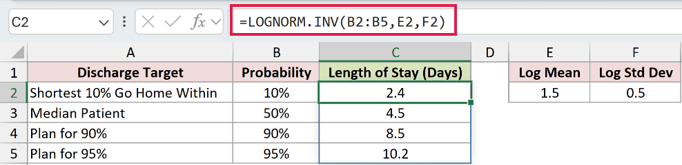
The probability range produces a spill into C2:C5. Each row uses the log mean of 1.5 and log standard deviation of 0.5.
The displayed thresholds are:
- 10%: 2.4 days.
- 50%: 4.5 days.
- 90%: 8.5 days.
- 95%: 10.2 days.
Under this model, 90% of stays fall at or below approximately 8.5 days. This is the percentile threshold for that discharge target.
Range formulas spill in Excel 2021, Excel 2024 and Microsoft 365. In Excel 2019 and earlier, use a per-row version and fill it down, keeping the parameter references fixed.
Pro Tip: Keep C3:C5 empty before entering the formula in C2. Existing content in the output range causes a #SPILL! error.
Example 2: Separate the Median From the Average
The middle percentile and the average aren’t the same in this model.
Below is the dataset. B1:B2 contain the log parameters, and the labelled cells beneath them will hold the median, average, and percentile comparisons.
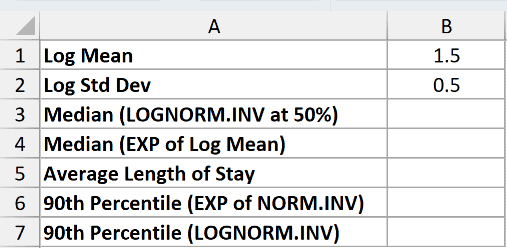
We want to compare the median with the actual model average and check an equivalent way to calculate a percentile.
Calculate the median in B3:
=LOGNORM.INV(0.5,B1,B2)
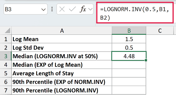
The result is 4.48 days. Using a probability of 50% returns the median, even though the argument name includes the word mean.
For the median equivalence check, enter this in B4:
=EXP(B1)
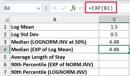
This check also returns 4.48 days. Taking EXP of the log mean recovers the median on the original scale.
Calculate the actual average length of stay in B5:
=EXP(B1+B2^2/2)
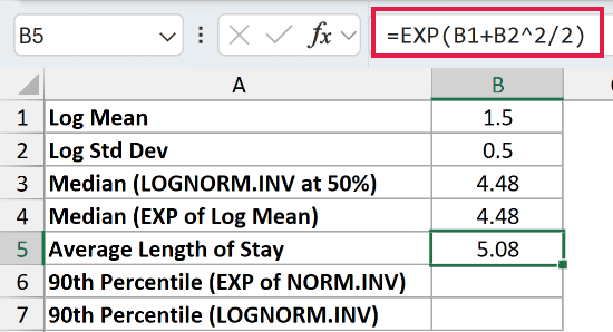
The model average is 5.08 days, higher than the 4.48-day median. The long upper tail pulls the average upward.
Next, enter the percentile equivalence check in B6:
=EXP(NORM.INV(0.9,B1,B2))
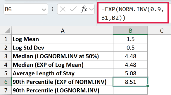
This comparison returns 8.51 days. NORM.INV finds the percentile on the log scale, and EXP converts it back to days.
Use LOGNORM.INV directly in B7:
=LOGNORM.INV(0.9,B1,B2)
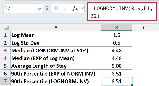
The direct formula also returns 8.51 days. B6 is an equivalence check; LOGNORM.INV performs the calculation without needing the outer EXP function.
Example 3: Start With a Known Median
You may know a model’s median before you know its log mean.
Below is the dataset. B1:B2 hold the median household income and log spread, with labelled cells for the log mean, median check, income percentile, and upper-tail share.
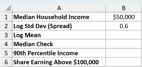
We want the 90th percentile of a sample income model with a $50,000 median and log standard deviation of 0.6.
Convert the median to a log mean in B3:
=LN(B1)
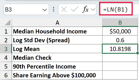
B3 displays 10.8198. LN reverses the EXP relationship from the previous example, giving us the mean argument LOGNORM.INV needs.
Check that the model returns the starting median in B4:
=LOGNORM.INV(0.5,B3,B2)
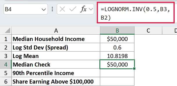
The check returns $50,000, matching the median input.
Calculate the 90th percentile income in B5:
=LOGNORM.INV(0.9,B3,B2)
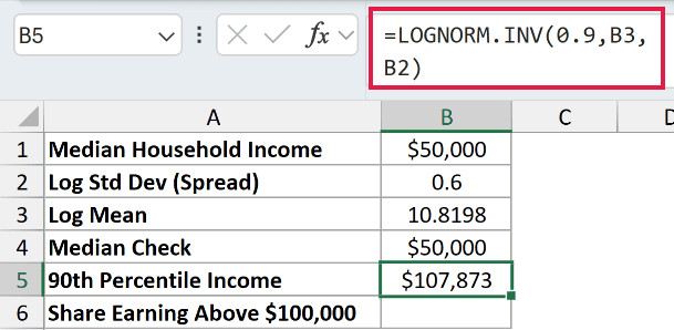
B5 displays $107,873. Under this sample model, 90% of household incomes fall at or below approximately that amount.
The reverse question starts with an income threshold and asks for a share. Use the sibling LOGNORM.DIST function in B6:
=1-LOGNORM.DIST(100000,B3,B2,TRUE)
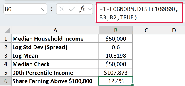
The result is 12.4%. LOGNORM.DIST returns the share at or below $100,000, so subtracting it from 1 returns the share above that threshold.
The spread in B2 is already a log-scale standard deviation. Knowing the median alone doesn’t determine that spread.
Example 4: Build a Lognormal Percentile Table
Now let’s generate the probabilities as well as their income thresholds.
Below is the dataset. D2:E2 contain the median income and log standard deviation; columns A and B provide space for percentile labels and income results.
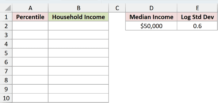
We want a decile table for the income model, with evenly spaced probabilities and their corresponding dollar amounts.
Generate the percentile labels in A2:
=SEQUENCE(9,1,0.1,0.1)
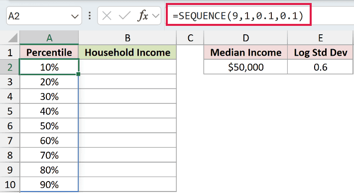
The formula spills into A2:A10. With percentage formatting, the labels run from 10% through 90%.
SEQUENCE requires Excel 2021 or later.
Calculate the income thresholds in B2:
=LOGNORM.INV(SEQUENCE(9,1,0.1,0.1),LN(D2),E2)
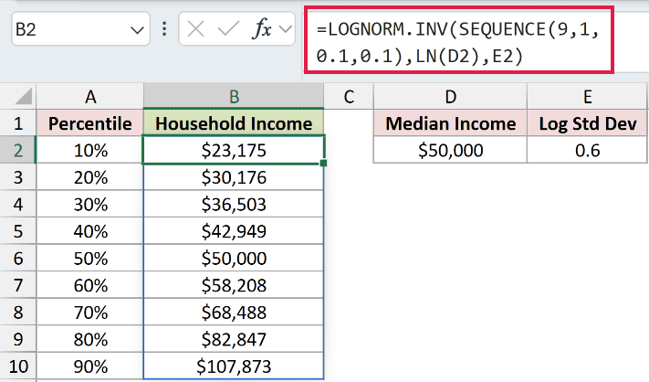
SEQUENCE supplies the probabilities inside LOGNORM.INV, while LN converts the median input to the log mean. The income results spill into B2:B10.
Here are the displayed results:
| Percentile | Household Income |
|---|---|
| 10% | $23,175 |
| 20% | $30,176 |
| 30% | $36,503 |
| 40% | $42,949 |
| 50% | $50,000 |
| 60% | $58,208 |
| 70% | $68,488 |
| 80% | $82,847 |
| 90% | $107,873 |
The probability steps are even, but the dollar gaps widen toward the upper tail.
Example 5: Estimate Parameters From Observed Stays
Let’s finish by calculating the log parameters from recorded lengths of stay.
Below is the dataset. A2:A8 contains stays in days; C2:D5 provides labelled cells for fitted parameters, a percentile estimate, and a deliberate raw-input mistake.
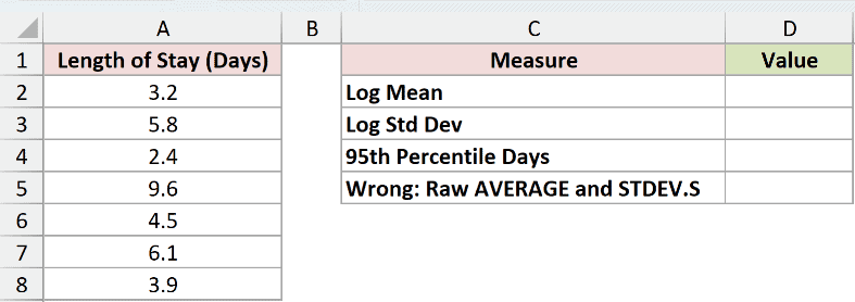
We want to estimate the 95th percentile using the logarithms of the observed stays.
Calculate the log mean in D2:
=AVERAGE(LN(A2:A8))
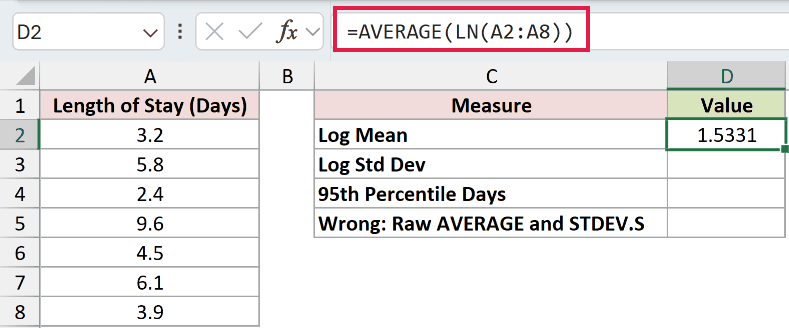
D2 displays 1.5331. LN transforms each stay before AVERAGE reduces those transformed values to a single mean.
Calculate the log standard deviation in D3:
=STDEV.S(LN(A2:A8))
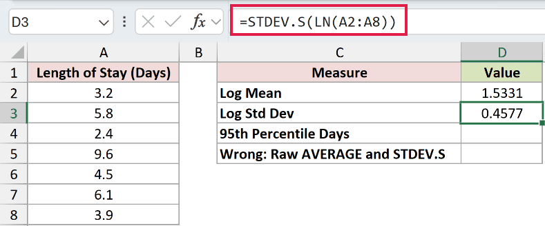
D3 displays 0.4577. STDEV.S measures the sample spread of the logarithms, rather than the spread of the original days.
These helper formulas each return a single value because AVERAGE and STDEV.S summarize the transformed array.
In Excel 2019 and earlier, confirm each helper formula with Ctrl+Shift+Enter.
Use those fitted parameters in D4:
=LOGNORM.INV(0.95,D2,D3)
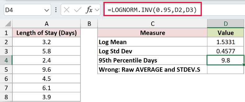
The estimated 95th percentile is 9.8 days. Referencing D2 and D3 keeps their stored precision, rather than substituting their rounded display values.
For the deliberate mistake in D5, the following formula passes the raw average and standard deviation directly into LOGNORM.INV:
=LOGNORM.INV(0.95,AVERAGE(A2:A8),STDEV.S(A2:A8))
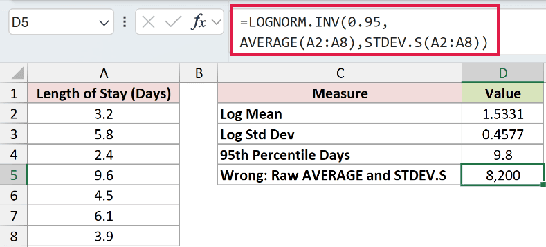
The mistake returns 8,200 days. D5 is an intentionally wrong result.
Excel treats those raw statistics as log-scale parameters. The formula runs without an error, but it describes the wrong distribution.
Pro Tip: Take the logarithms before calculating either parameter. In this example, D2 and D3 are the correct inputs; the raw-statistics formula in D5 is the mistake to avoid.
Tips & Common Mistakes
- Exclude the endpoints. A probability of 0 or 1 returns
#NUM!. Choose a probability strictly between them. - Check the spread. A zero or negative
standard_devreturns#NUM!. A negative log mean can still be valid. - Keep the direction straight. LOGNORM.INV turns a cumulative probability into a value. LOGNORM.DIST answers the reverse question using a value you already have.
- Don’t confuse the median with the average. The 50% result is the median. Example 2 calculates the model average separately.
- Use the log statistics. The inputs describe LN-transformed observations. Passing raw statistics can produce a plausible-looking formula with a wildly wrong answer.
- Keep model estimates distinct from observations. Example 5 calculates a percentile of the fitted lognormal model, rather than selecting a percentile directly from the recorded stays.
Related Excel Functions / Articles:
