
Excel’s MINA function returns the smallest value, treating TRUE as 1 and FALSE or text in worksheet references as 0.
That behavior makes MINA useful when labels such as “Out of stock” mean zero. It can also produce misleading answers when text means unknown or pending.
In this article, I’ll show you how MINA handles mixed cell types, why dates can display as 1/0/1900, and what changes inside FILTER.
MINA Function Syntax in Excel
The MINA function uses this syntax:
=MINA(value1, [value2], ...)
- value1 (required) is the first value, cell, or range you want MINA to evaluate.
- value2, … (optional) represents up to 254 additional values, cells, or ranges, for a maximum of 255 arguments in total.
When to Use MINA Function
- Find the smallest entry when TRUE, FALSE, or status text carries a numeric meaning.
- Treat labels such as “Out of stock” as zero while finding the lowest inventory level.
- Compare MINA with MIN when deciding whether text should count or be ignored.
- Check how MINA interprets numbers, logical values, text, and blanks in a mixed range.
Example 1: MINA vs MIN for Stock Markers
Here’s a stock list that shows where MINA and MIN differ.
Below is the dataset. Column A lists spare parts, column B holds stock counts or status text, and two labeled cells will show the lowest stock.
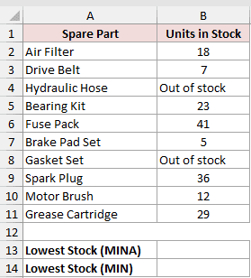
We want to see how MINA and MIN handle the “Out of stock” entries.
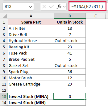
Here is the MINA formula:
=MINA(B2:B11)
And here is the MIN formula for comparison:
=MIN(B2:B11)
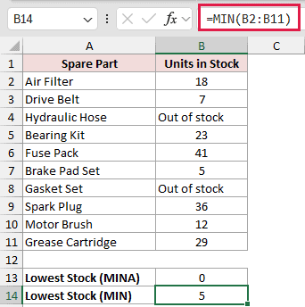
MINA returns 0 because “Out of stock” is text in a referenced range. MIN returns 5 because it ignores those text entries.
Here, zero is the useful answer because the text describes a real stockout. If the text meant unavailable data, MIN would be the better choice.
Example 2: How MINA Treats Cell Types
This next example isolates each conversion rule.
Below is the dataset. Column A describes each entry, column B holds the entry itself, and column C will hold the MINA result copied down the rows.
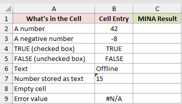
We want to see what MINA returns when each entry is referenced individually.
Enter this formula in C2 and copy it down through C9:
=MINA(B2)
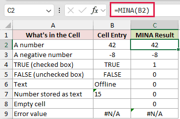
The number 42 stays 42, and -8 stays -8. TRUE returns 1, while FALSE and the text “Offline” each return 0.
The number stored as text, 15, also returns 0. The empty cell in B8 returns 0 when it is the only referenced input.
The #N/A placeholder in B9 passes through to C9. MINA does not skip an error value the way it skips an empty cell.
Example 3: Avoid 1/0/1900 in Date Results
Here’s the opposite case, where treating text as zero gives the wrong answer.
Below is the dataset. It lists vehicles, assigned drivers, and service dates or “TBD” markers, with two labeled cells waiting for the earliest date.
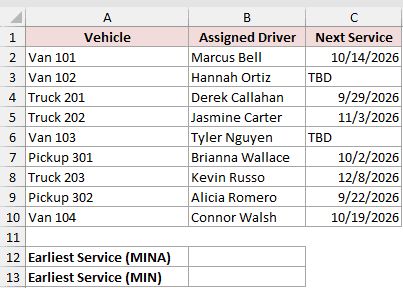
We want to find the earliest scheduled service without treating “TBD” as a real date.
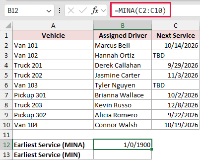
Here is the MINA formula:
=MINA(C2:C10)
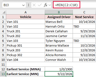
And here is the MIN formula:
=MIN(C2:C10)
MINA converts the “TBD” text to 0. Because B12 uses a date format, that zero appears as 1/0/1900.
The display can look different with other regional date settings.
MIN ignores the “TBD” entries and returns 9/22/2026, the earliest actual service date in the list.
Pro Tip: A 1/0/1900 result in a date column can be a zero wearing a date format. Check whether a text placeholder was converted to 0.
Example 4: Avoid the MINA With FILTER Trap
The last example finds the lowest stock for one vending location.
Below is the dataset. It lists machines, snacks, and units left. Two labeled result cells sit below it, and white cell B15 will demonstrate the mistake.
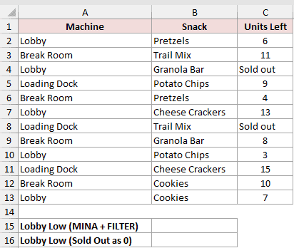
We want Lobby’s lowest stock while counting “Sold out” as zero.
Here is the tempting MINA and FILTER formula:
=MINA(FILTER(C2:C13,A2:A13="Lobby"))
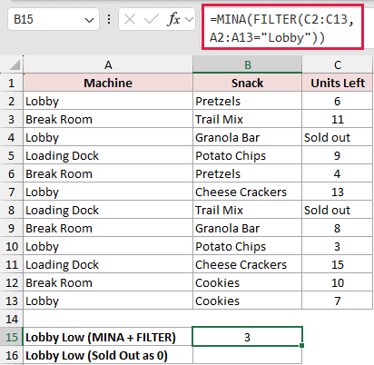
That formula returns 3, which is the deliberate mistake shown in white cell B15.
FILTER creates a computed array. Inside that array, MINA ignores text and logical values just as MIN does, so “Sold out” disappears from the calculation.
Here is the corrected formula:
=MIN(FILTER(IF(ISTEXT(C2:C13),0,C2:C13),A2:A13="Lobby"))
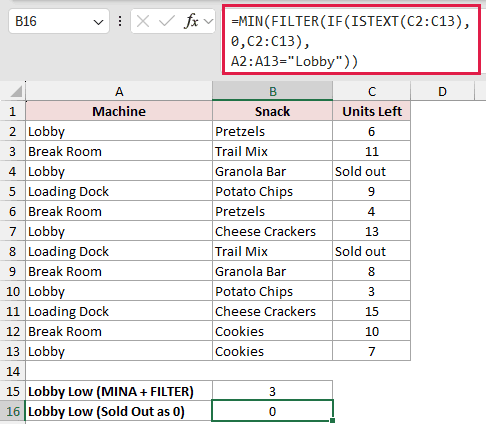
ISTEXT identifies the text entries. IF converts each one to 0 before FILTER builds the Lobby subset.
MIN then returns the intended result of 0 in B16.
FILTER is available in Excel 2021 and later. MINA still returns a single value here because it reduces the filtered array.
Tips & Common Mistakes
- MINA returns one result and does not spill by itself, even when you pass it a range.
- In worksheet references, TRUE counts as 1, while FALSE and text count as 0. Empty cells are ignored when other values remain.
- A reference containing only an empty cell returns 0 because MINA has nothing else to evaluate. Make sure that zero is meaningful before using it.
- Errors pass through. A #N/A input produces a #N/A result rather than being ignored.
- There is no MINAIFS function. MINIFS ignores text, so it cannot reproduce MINA’s text-as-zero behavior for conditional calculations.
- Typed arguments behave differently from references.
=MINA(5,TRUE)returns 1, while=MINA(5,"TRUE")returns#VALUE!. - Computed arrays ignore text and logical values. For example,
=MINA({5,TRUE,"x"})returns 5, so convert meaningful text to 0 first. =MINA(B2:E2)returns 1 only when every checkbox value is TRUE, but=AND(B2:E2)states that test more clearly.
MINA is a small function, but its zeros often reveal something important about the source data.
If a result looks surprising, inspect the underlying cell types before changing the formula.
Related Excel Functions / Articles:
