
The PERCENTOF function in Excel returns the share that a subset represents of a total. It adds the subset’s values and divides by the sum of the complete set.
You can use it to measure one item’s contribution or summarize percentages by category. A result of 0.25 means the subset accounts for 25% of the total.
In this article, I’ll show you how to calculate individual shares, measure filtered subsets, and build percentage summaries with GROUPBY and PIVOTBY.
PERCENTOF Function Syntax in Excel
PERCENTOF has two required arguments:
=PERCENTOF(data_subset,data_all)
data_subsetcontains the number or values whose share you want to calculate.data_allcontains the complete set of values used as the denominator.
Both arguments can contain multiple values. PERCENTOF adds each set before dividing, so a range argument produces one combined share rather than a separate percentage for every row.
PERCENTOF is available in Microsoft 365. If your Excel version doesn’t support it, divide the subset’s sum by the complete set’s sum instead.
When to Use PERCENTOF Function
- Calculate each item’s contribution to a total.
- Measure the share associated with records meeting a condition.
- Summarize category shares with GROUPBY.
- Compare percentage contributions across two categories with PIVOTBY.
- Calculate each text category’s share of a record count.
Example 1: Calculate Each Item’s Share
Let’s start with individual contributions to a total.
Below is the dataset with volunteer hours for six trail sections and an empty Share of All Hours column.
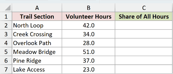
I want to calculate each trail section’s share of the total volunteer hours.
Here is the formula in C2, filled down through C7:
=PERCENTOF(B2,$B$2:$B$7)
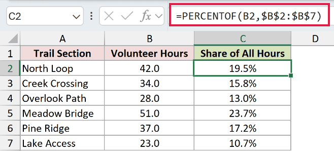
The six sections total 215 hours. North Loop contributes 42 hours, so C2 displays 19.5% when formatted as a percentage with one decimal place.
The remaining shares are 15.8%, 13.0%, 23.7%, 17.2%, and 10.7%. Each percentage compares one section with the same 215-hour total.
The dollar signs keep the denominator fixed as the formula is copied down. The first argument changes from B2 to B3, B4, and so on.
Passing the entire hours column as the first argument would combine those hours. It would return the whole set’s share, not six individual percentages.
Pro Tip: Apply Percentage formatting to the result cells. PERCENTOF returns a decimal ratio; multiplying by 100 as well as applying Percentage formatting would make the displayed percentage too large.
Example 2: Measure a Filtered Subset
A subset can contain records scattered throughout a list.
Below is the dataset with 12 support tickets, their resolution statuses, and hours billed. The separate result cell will show the completed-work share.
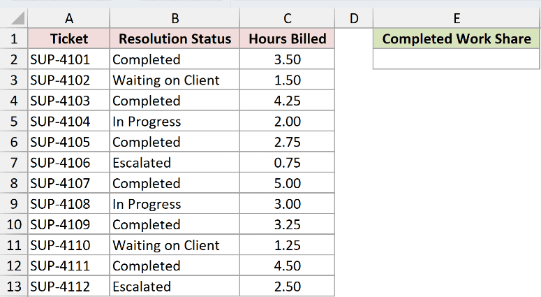
I want to find what percentage of billed hours belongs to completed tickets.
Here is the formula in E2:
=PERCENTOF(FILTER(C2:C13,B2:B13="Completed"),C2:C13)
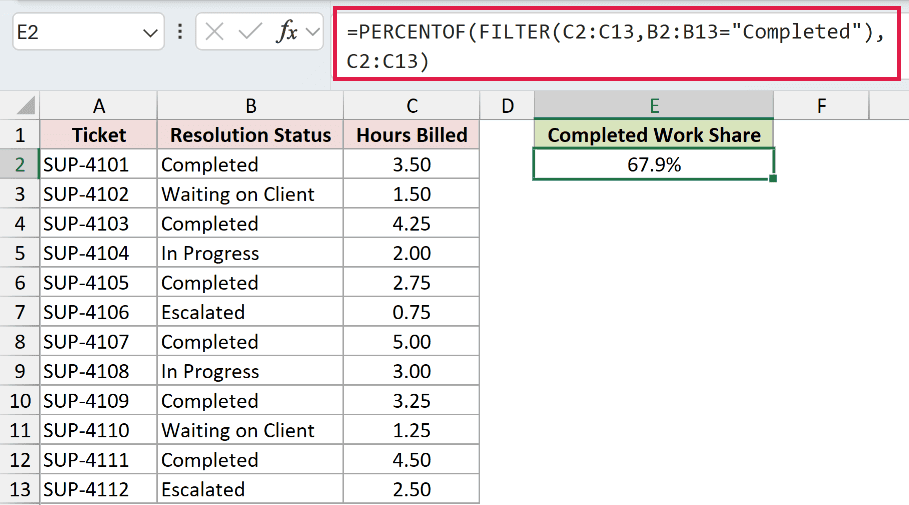
The FILTER function returns the hours from rows whose status is Completed. PERCENTOF adds those hours and compares them with all hours in C2:C13.
Completed tickets account for 23.25 of the 34.25 billed hours. E2 therefore displays 67.9%.
This measures the share of hours, not the share of tickets. A five-hour ticket contributes more to the result than a one-hour ticket.
Although FILTER returns several values inside the formula, PERCENTOF combines them into one result. There is no output list spilling from E2.
Pro Tip: This example contains completed tickets. If none match, FILTER returns a #CALC! error without its optional empty-result argument. Decide how an empty subset should be handled before adapting the formula.
Example 3: Summarize Percentages by Category
PERCENTOF can also calculate shares within a grouped summary.
Below is the dataset with 12 repair work orders, their categories, and billed amounts. Columns E and F provide space for the summary.
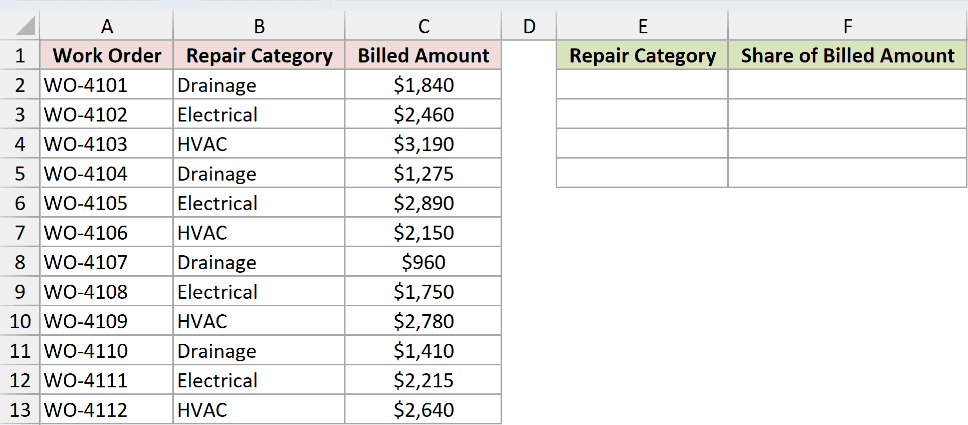
I want one percentage for each repair category, measured against all billed work.
Here is the formula in E2:
=GROUPBY(B2:B13,C2:C13,PERCENTOF)
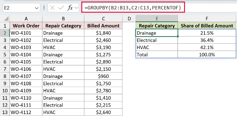
The GROUPBY function groups the billed amounts by repair category. Its third argument selects PERCENTOF as the calculation for each group.
Notice that PERCENTOF has no parentheses here. GROUPBY passes the group’s values and the comparison values to it, rather than requiring a separate PERCENTOF formula for each category.
The billed amounts total $25,560. Drainage contributes $5,485, Electrical contributes $9,315, and HVAC contributes $10,760.
The spilled summary displays 21.5%, 36.4%, and 42.1%, respectively. Its Total row displays 100.0%.
The formula occupies E2, but its output extends through F5. Changing a source amount updates the grouped percentages.
Pro Tip: Keep the summary area clear. Typing into the cells needed by a dynamic-array result causes a #SPILL! error.
Example 4: Build a Two-Way Percentage Summary
You can break the total down by two categories at once.
Below is the dataset with transit grants, project phases, and allocated amounts. The empty area on the right will hold the percentage summary.
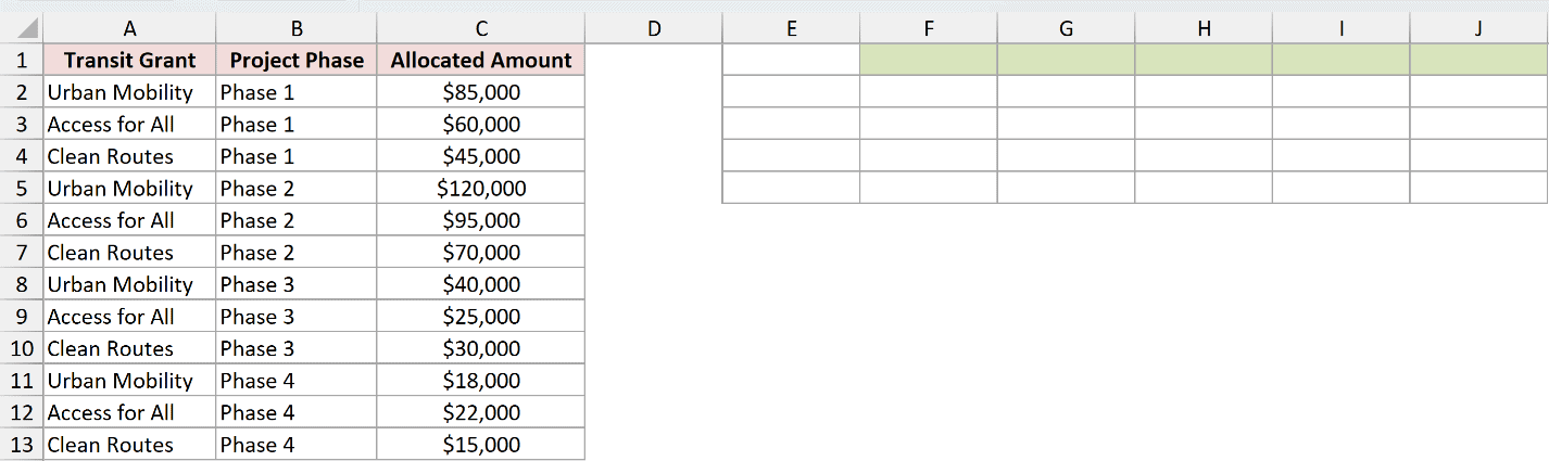
I want each grant-and-phase combination expressed as a share of all allocated funding.
Here is the formula in E1:
=PIVOTBY(A2:A13,B2:B13,C2:C13,PERCENTOF,,,,,,,2)
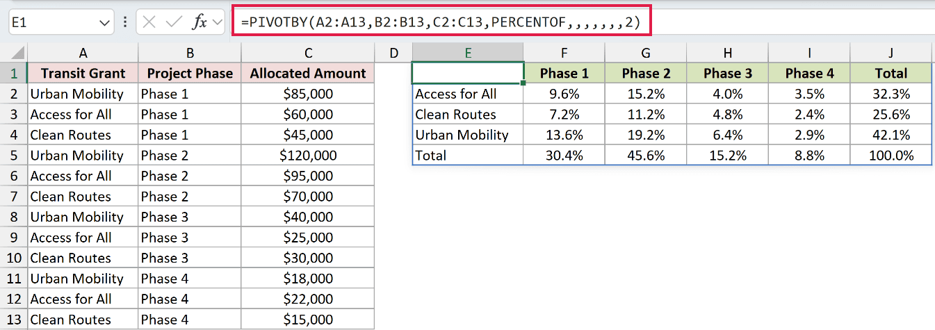
The PIVOTBY function places grant names down the rows and project phases across the columns. PERCENTOF calculates the percentage values inside that grid.
How this formula works:
- A2:A13 supplies the row groups: the transit grants.
- B2:B13 supplies the column groups: the project phases.
- C2:C13 supplies the allocated amounts.
- PERCENTOF calculates shares instead of returning the summed dollar amounts.
- The final 2 sets
relative_toto the grand total. The intervening optional arguments use their defaults.
All allocations total $625,000. Access for All receives $60,000 in Phase 1, so that intersection displays 9.6% of the grand total.
The Total column shows 32.3% for Access for All, 25.6% for Clean Routes, and 42.1% for Urban Mobility.
The bottom row shows each phase’s share of all funding: 30.4%, 45.6%, 15.2%, and 8.8%. The bottom-right cell displays 100.0%.
Pro Tip: Choose the denominator deliberately. A share of the grand total answers a different question from a share of one row or column. Here, the final 2 explicitly selects the grand total.
Example 5: Calculate Shares of Text Categories
Sometimes each record should count equally, regardless of any dollar amount or duration.
Below is the dataset with 12 visitor registrations and their registration channels. Columns D and E are reserved for the category shares.
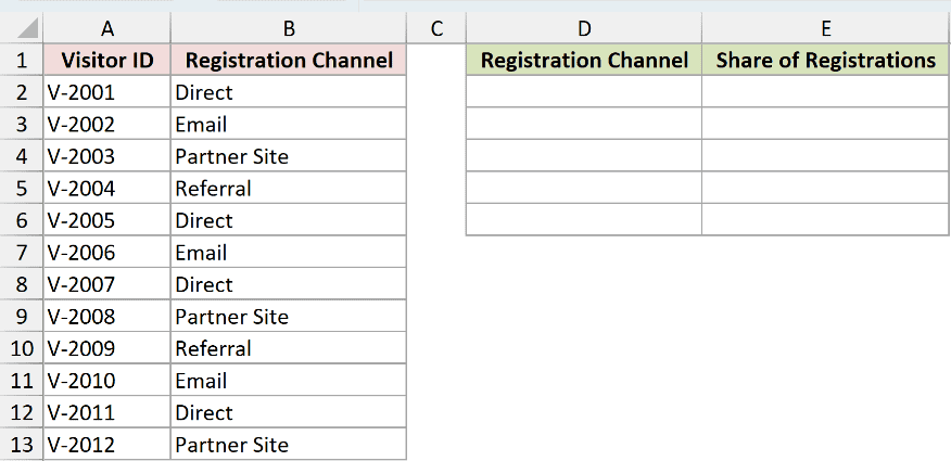
I want each channel’s share of the total number of registrations.
Here is the formula in D2:
=GROUPBY(B2:B13,SEQUENCE(ROWS(B2:B13),,1,0),PERCENTOF)
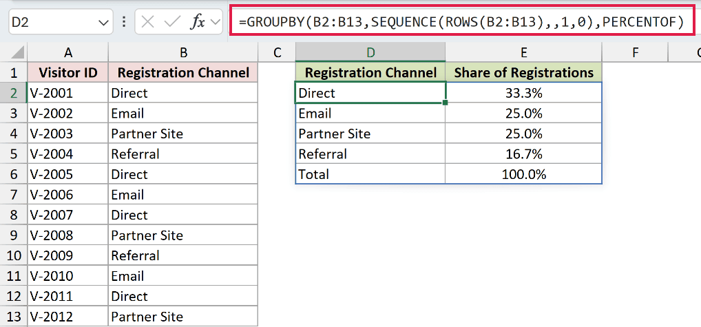
The registration channels are text labels. To calculate their shares by count, the formula assigns a numeric value of 1 to each registration.
How this formula works:
- ROWS counts the 12 rows in B2:B13.
- The SEQUENCE function creates 12 values, starting at 1 with a step of 0. Every value is therefore 1.
- GROUPBY groups those ones by registration channel.
- PERCENTOF compares each group’s total with all 12 ones.
Direct has four registrations, Email has three, Partner Site has three, and Referral has two. The summary displays 33.3%, 25.0%, 25.0%, and 16.7%.
The Total row displays 100.0%. Because every row contributes 1, the percentages describe registration counts rather than the sum of another measure.
Pro Tip: Keep the generated ones array the same length as the category range. Using ROWS ties its size to the range instead of hard-coding the record count.
Tips & Common Mistakes
- PERCENTOF returns a ratio. Use Percentage formatting to display it as a percentage.
- The denominator’s sum must not be zero. A zero denominator produces a #DIV/0! error.
- Lock the total range when filling a row-by-row formula down a list.
- A multi-cell subset is summed into one share. It does not produce an individual result for every value.
- Use numeric measures for grouped shares. To measure text-category counts, supply one numeric unit per record as in Example 5.
- Check the comparison total when using PIVOTBY. Percentages of a row, column, and grand total have different meanings.
- Displayed rounded percentages may not add up to exactly 100%. Excel retains more precision than the one-decimal display shown here.
- These examples require Microsoft 365 with the functions available. For older Excel, use sums and division, or a PivotTable percentage-of-total calculation.
I covered individual contributions, a filtered subset, and percentage summaries by one or two categories. The final example showed how to calculate shares when each record counts equally.
I hope you found this article helpful.
Related Excel Functions / Articles:
