
If you want to forecast next year’s sales but a single “best guess” number feels shaky, a Monte Carlo simulation gives you a range instead.
The idea is simple. Instead of one forecast, you run the same model hundreds of times with random inputs and look at the spread of results.
Desktop Excel for Windows and Mac handles this without add-ins or VBA. In this tutorial, I’ll build the model from scratch on two years of monthly sales, using RAND, NORM.INV, and a Data Table to run the trials.
Step 1: Set Up the Sales Assumptions and Historical Data
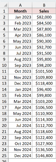
This simplified demonstration estimates its inputs from two years of monthly sales, running from January 2023 through December 2024.
It treats each month’s log growth as an independent draw from the same distribution. It does not model seasonality, trend, autocorrelation, or structural changes.
Below is the dataset. Column A has the month and column B has the sales for that month.
The model uses log growth, the natural log of the ratio between consecutive months. Log growth works cleanly with exponential compounding and helps keep every simulated sales value positive.
In cell C3, I enter this formula and copy it down to the last month:
=LN(B3/B2)
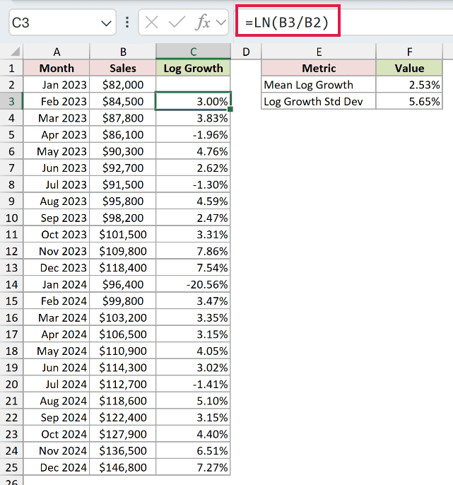
A positive result means sales rose, while a negative result means they fell. I then summarize the log-growth values with their mean and sample standard deviation.
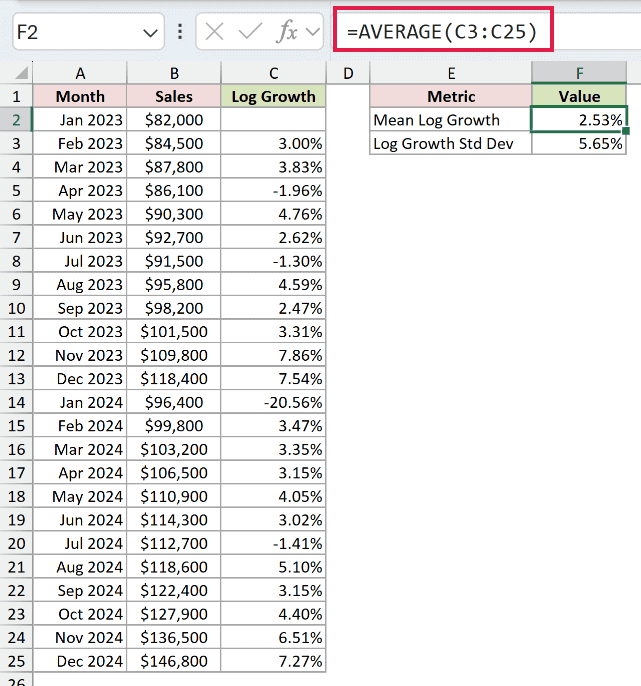
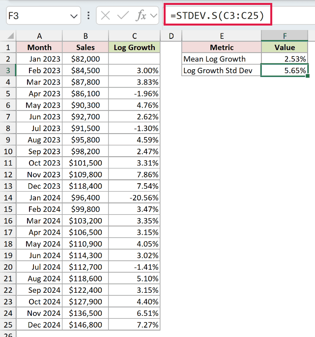
In cell F2, I calculate the mean monthly log growth. In F3, I calculate the sample standard deviation of log growth:
=AVERAGE(C3:C25)
Here is the standard deviation formula in cell F3:
=STDEV.S(C3:C25)
How does this work?
AVERAGE gives the arithmetic mean of the monthly log-growth values. STDEV.S estimates their sample standard deviation, so a larger value means the historical log growth was more dispersed.
Together, these cells provide the two parameters for the normal log-growth distribution used in this demonstration.
Step 2: Generate Random Sample Values With RAND and NORM.INV
Now each simulated month gets a random log-growth value from the normal distribution defined in Step 1. The model draws each month separately and treats the draws as independent.
The pair of functions that does this is RAND and NORM.INV. Here’s the formula for one random log-growth value:
=NORM.INV(RAND(),$F$2,$F$3)
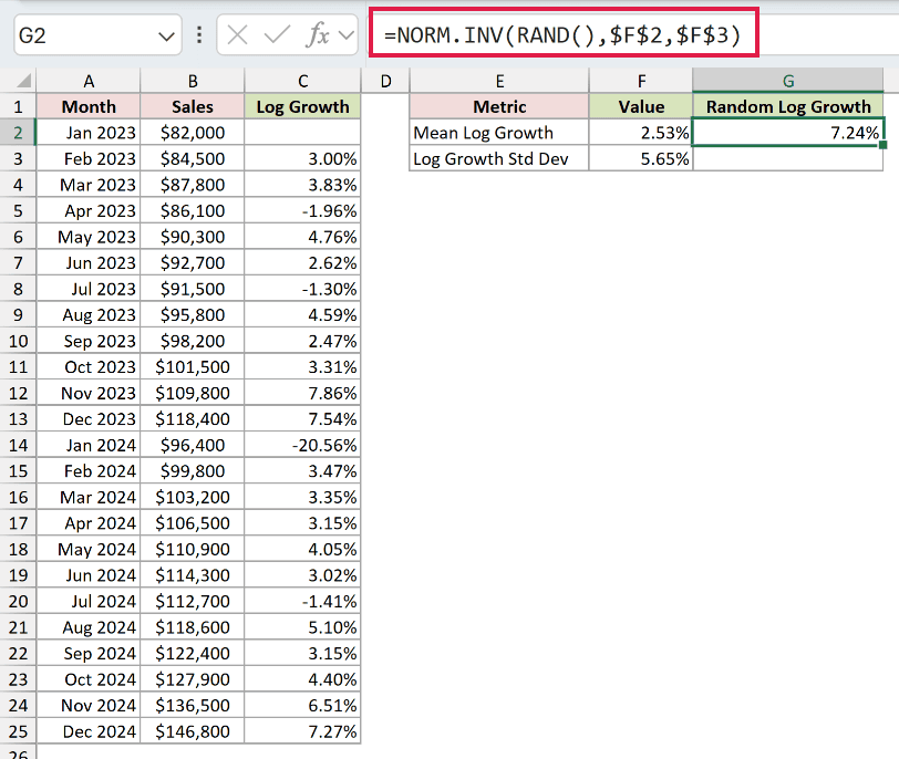
How does this formula work?
RAND() spits out a random decimal between 0 and 1, with every value equally likely. On its own that’s a flat, featureless spread.
NORM.INV maps that probability to a normal distribution. Its three inputs are the RAND probability, the mean log growth in F2, and the sample standard deviation in F3.
The result uses the mean and spread estimated from this history. It is still only a simplified model, because the distribution and independent-month assumptions may not describe future sales.
Note: RAND is volatile, so it produces new values when Excel recalculates or you press F9. Standard worksheet use does not provide a user-set seed. Paste-values can freeze one run, but it cannot reproduce that run later.
Step 3: Build the Simulation Model
A single simulation run is one possible version of next year. I’ll project 12 months forward, where each month grows on the previous one by a fresh random rate from Step 2.
I set this up in a small block to the side. Cell H1 holds the starting point, the last actual sales figure from December 2024:
=B25
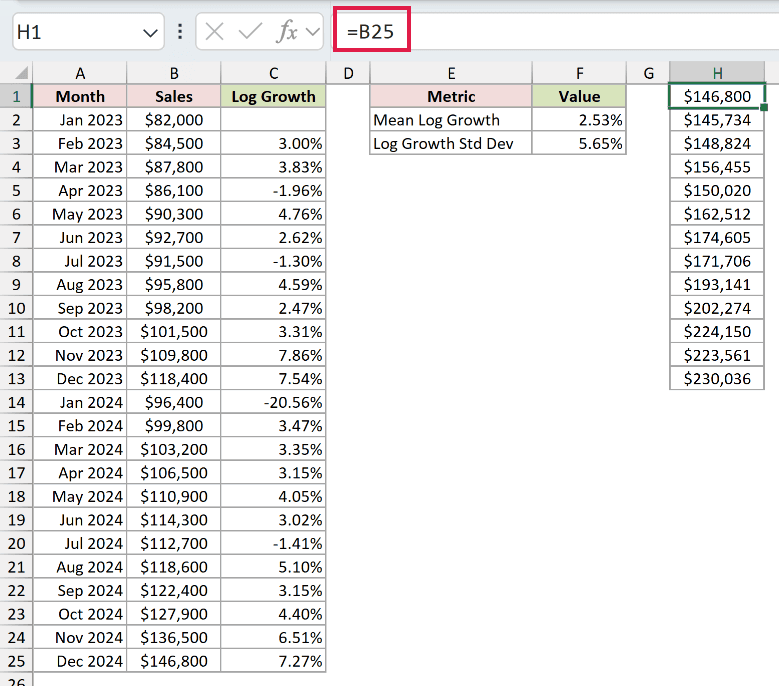
Then, in H2, I apply the random log growth through EXP to create a positive monthly multiplier:
=H1*EXP(NORM.INV(RAND(),$F$2,$F$3))
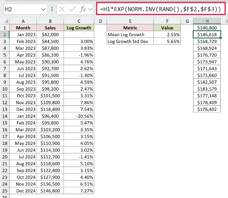
I copy H2 down through H13 to cover all 12 months. Each row compounds from the row above, so an earlier draw affects later sales levels. That is compounding and path dependence, not momentum.
Finally, in cell K1, I total the 12 forecast months to get this run’s projected annual sales:
=SUM(H2:H13)
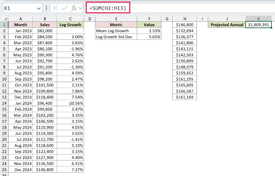
How does this work?
Cell K1 is the single output I care about, the total sales for the whole simulated year. Every time Excel recalculates, all those RAND-driven months redraw, and K1 lands on a different total.
Press F9 a few times and you’ll watch it jump around. Depending on your Mac keyboard settings, you may need Fn + F9. Each recalculation produces another scenario under the same model assumptions.
Step 4: Run Multiple Trials With a Data Table
Pressing F9 by hand and jotting down numbers would take forever. In desktop Excel, a Data Table can evaluate the model repeatedly and record each recalculated result in a column.
First, I set up a list of trial numbers. In cell M2 I type 1, in M3 I type 2, and fill down to 500 to run 500 trials.
Then, one cell up and one to the right, in N1, I point to my model’s output:
=K1
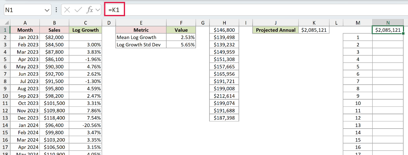
Now I select M1:N501, including the empty corner, trial numbers, and formula. Microsoft documents creating Data Tables in desktop Excel for Windows and Mac. Use desktop Excel to build this table.
Here are the steps:
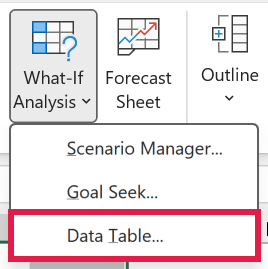
- With the range M1:N501 selected, go to the Data tab and click What-If Analysis, then Data Table.
- Leave the Row input cell box empty. In the Column input cell box, click any blank cell that your model doesn’t use (I picked an empty cell like P1), then click OK.
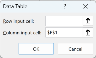
Excel fills column N with 500 annual totals, one per trial. Each row records a separately recalculated scenario from the model.
How does this work?
Microsoft’s documented one-variable Data Table pattern expects the output formula to depend on one input cell. This example uses a volatile-model workaround: the trial numbers are substituted into blank, unused P1.
The output does not depend on P1. The substitution triggers another evaluation, and RAND supplies fresh draws. The trial column provides 500 rows for separately recalculated scenarios.
Note: In Windows desktop Excel, go to File > Options > Formulas and choose Partial, which recalculates automatically except for Data Tables. On Mac, go to Excel > Preferences > Calculation and choose Automatically except for data tables. Press F9 when you want new trials.
Step 5: Analyze the Simulation Results
The 500 numbers in column N are the simulated outcomes. I’ll summarize their center and central 90% under this model’s assumptions.
I start with the mean, which is the arithmetic average of all 500 simulated annual totals:
=AVERAGE(N2:N501)
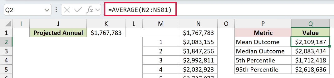
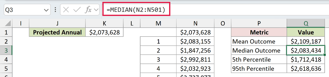
I also calculate the median, the middle simulated total after the outcomes are sorted:
=MEDIAN(N2:N501)
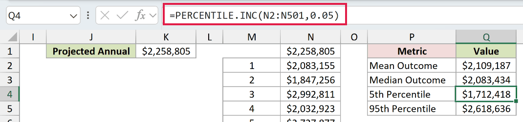
Next, I use PERCENTILE to find the endpoints of the central 90% of simulated outcomes. Here is the 5th percentile:
=PERCENTILE.INC(N2:N501,0.05)
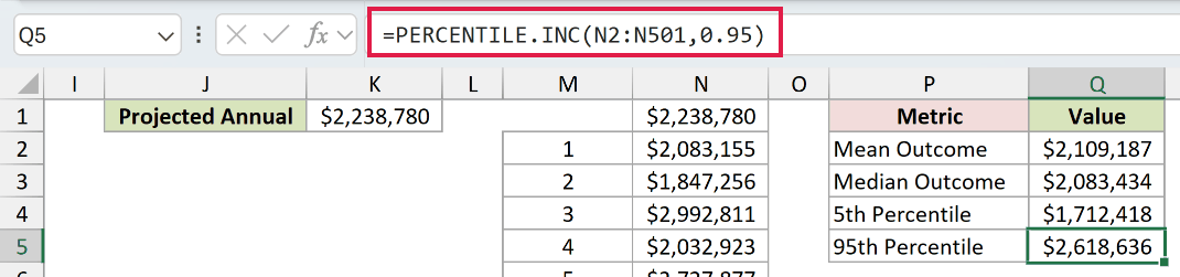
Here is the 95th percentile in the next cell:
=PERCENTILE.INC(N2:N501,0.95)
How does this work?
AVERAGE gives the simulation mean, while MEDIAN gives its middle outcome. They can differ when the simulated totals are skewed.
The 5th and 95th percentiles bound the central 90% of these simulated outcomes, conditional on the model assumptions. This is not a statistical confidence interval.
You can report that central simulated range, but the actual future can fall outside it, and the model assumptions themselves can be wrong.
To see the shape of the outcomes, I select the results in column N and insert a histogram. Go to the Insert tab, click the statistic chart icon, and choose Histogram:
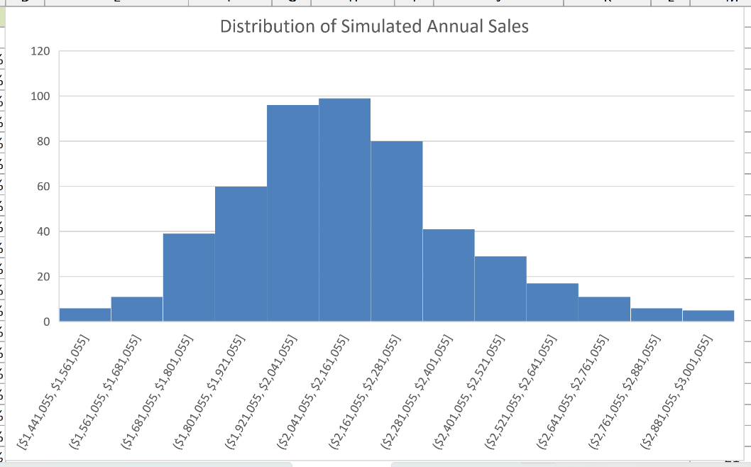
The histogram groups the trials into buckets and shows how many landed in each. You’ll usually see a hump in the middle where most outcomes cluster, with thin tails on either side.
The histogram shows the distribution generated by the model. It does not prove that the model assumptions describe future sales correctly.
Additional Notes About Monte Carlo Simulation in Excel
- The assumptions define the result. This demonstration ignores seasonality, trend, autocorrelation, and structural changes. A real forecasting model should test and model those features when they matter.
- The distribution is a modeling choice. This example assumes normal log growth, which makes the monthly sales multiplier lognormal and keeps sales positive. Check whether that assumption fits your data.
- Freezing is not reproducing. Paste Special as Values preserves one set of outcomes for a report, but standard worksheet RAND offers no user-set seed for recreating it later.
- Use more trials for stable tails. Five hundred trials works for this demonstration. For more stable 5th and 95th percentiles, use thousands and check whether the summaries converge across recalculations.
Frequently Asked Questions
How many trials do I need for a reliable Monte Carlo simulation?
There is no universal number. Five hundred trials is fine for this demonstration, but tail estimates such as the 5th and 95th percentiles usually benefit from thousands of trials.
Increase the trial count and repeat the simulation until the mean, median, and percentiles change only slightly. That convergence check is more useful than relying on one fixed rule.
Why does my Monte Carlo simulation change every time I open the file?
RAND is volatile and redraws when Excel recalculates, including when the workbook opens. Standard worksheet RAND has no user-set seed. Pasting the results as values freezes that run, but it does not make the run reproducible.
Can I run a Monte Carlo simulation without VBA?
Yes, and this whole tutorial does exactly that. RAND, NORM.INV, and a Data Table handle everything with native worksheet features. VBA can help automate very large or repeated studies, but it isn’t required for a standard simulation.
Conclusion
In this tutorial, I used historical log growth, positive exponential compounding, a Data Table, and mean, median, and percentile summaries to demonstrate Monte Carlo simulation in Excel.
The results are conditional on a deliberately simple model, so check the assumptions and convergence before using the tails for a real decision.
I hope you found this article helpful!
Other Excel articles you may also like:
