How to Transpose Multiple Rows into One Column in Excel

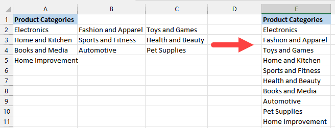
At times, you might need to transpose or change your Excel data from several rows into a single column, as shown below:

Here, I got data in separate rows, and I had to not only convert that data from rows to columns but also combine the data from all the separate rows.

This is something I often need to do when I get my data from external sources, which are in different rows, and I need all the data transposed in a column where all the rows of data are combined in a single column.

This tutorial shows four techniques for transposing multiple rows of data into a single column in Excel.

Method #1: Using INDEX, COLUMNS, INT, and MOD Functions

In Excel, you can use a formula that combines the INDEX, COLUMNS, INT, and MOD functions to transpose multiple rows of data into a single column.

Let’s say we have the following dataset that displays the product categories of an online store arranged in multiple rows:

We aim to use a formula that combines the INDEX, COLUMNS, INT, and MOD functions to convert the data from multiple rows into a single column.

We use the following steps:

1. Name the data range by doing the following:
   • Select the cell range A2:C5, right-click the selection, and choose “Define Name” from the shortcut menu.

• On the “New Name” dialog box, enter a name on the “Name” field, ensuring no spaces in the name. In this case, we enter “Product_Categories” and click “OK.”

2. Select a blank cell on the worksheet (in this example, we have selected cell E2) and enter the following formula:

=INDEX(Product_Categories,1+INT((ROW(A1)-1)/COLUMNS(Product_Categories)),MOD(ROW(A1)-1+COLUMNS(Product_Categories),COLUMNS(Product_Categories))+1)

3. Drag the fill handle in cell E2 to copy the formula down the column.

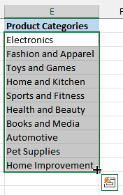
As depicted below, the data that was once spread across several rows has now been combined into a single column:

Explanation of the Formula

=INDEX(Product_Categories,1+INT((ROW(A1)-1)/COLUMNS(Product_Categories)),MOD(ROW(A1)-1+COLUMNS(Product_Categories),COLUMNS(Product_Categories))+1)

The Excel formula uses the INDEX function to retrieve values from the range  “Product_Categories” in a structured manner, cycling through rows and columns within the range.

Here’s a breakdown of the formula:

1. ROW(A1)-1: This calculates the current row number minus one. The ROW function returns the row number of a cell reference, and in this case, we subtract one to make it zero-based.
2. COLUMNS(Product_Categories): This returns the number of columns in the “Product_Categories” range.
3. ROW(A1)-1/COLUMNS(Product_Categories): This division calculates the relative row position within the range. For example, if the range has three columns, it determines which “row group” the current row belongs to.
4. 1+INT((ROW(A1)-1)/COLUMNS(Product_Categories)): The INT function rounds down the result of the previous division, and then 1 is added, giving us the group number of the current row.
5. ROW(A1)-1+COLUMNS(Product_Categories): This adds the current row number minus one to the number of columns in the range. It helps in creating a repeating sequence of numbers.
6. MOD(ROW(A1)-1+COLUMNS(Product_Categories),COLUMNS(Product_Categories))+1: The MOD function calculates the remainder when the previous sum is divided by the number of columns. The result is then incremented by one, giving us the column position within the group.
7. INDEX(Product_Categories, … ): Finally, the INDEX function takes the “Product_Categories” range and retrieves the value at the specified row and column positions.

Also read: How to Convert Columns to Rows in Excel?

Method #2: Using OFFSET, ROUNDUP, ROWS, and MOD Functions

In Excel, you can utilize a formula that integrates the OFFSET, ROUNDUP, ROWS, and MOD functions to transpose multiple rows of data into a single column.

Imagine we have a dataset showing the product categories of an online store arranged in several rows:

We aim to use a formula that combines the OFFSET, ROUNDUP, ROWS, and MOD functions to convert the data from multiple rows into a single column.

We use the below steps:

1. Select a blank cell on the worksheet (in this example, we have selected cell E2) and enter the following formula:

=OFFSET($A$2,ROUNDUP(ROWS($1:1)/3,0)-1,MOD(ROWS($1:1)-1,3))

2. Drag the fill handle in cell E2 to copy the formula down the column.

The data that was previously in multiple rows has been consolidated into a single column, as shown below:

Explanation of the Formula

=OFFSET($A$2,ROUNDUP(ROWS($1:1)/3,0)-1,MOD(ROWS($1:1)-1,3))

The Excel formula dynamically retrieves data from a range.

Here’s a breakdown of the formula:

1. $A$2: This is the starting cell reference. It represents the cell from which the OFFSET function will begin retrieving data.
2. ROWS($1:1): This expression calculates the current row number relative to the range $1:1. As the formula is copied down, the row number increases, allowing the OFFSET function to move to different rows.
3. ROUNDUP(ROWS($1:1)/3,0)-1: This part divides the current row number by 3 and rounds it up to the nearest whole number. It determines the number of rows to offset from the starting cell. Subtracting 1 ensures that the offset is relative to the starting cell, which is A2.
4. MOD(ROWS($1:1)-1,3): The MOD function calculates the remainder of the division operation (ROWS($1:1)-1)/3. It determines the number of columns to offset from the starting cell. The ROWS($1:1)-1 expression subtracts 1 from the row number, and then the MOD function returns the remainder when divided by 3.

By combining these calculations, the formula effectively offsets the cell reference by a variable number of rows and columns, allowing you to retrieve data from a range in a pattern of three rows and three columns.

As you copy the formula down, the ‘ROWS($1:1)’ part increases, resulting in a different offset for each row, effectively fetching data from another cell based on the pattern defined by the formula.

Also read: How to Reverse a Text String in Excel (Using Formula & VBA)

Method #3: Using Power Query to Transpose Multiple Rows into One Column

With Power Query, we can convert data that spans multiple rows into a single column.

Let’s consider a dataset that displays the product categories of an online store in multiple rows.

We want to use Power Query to transpose the data into a single column.

We use the steps below:

1. Convert the data range to a table by doing the following:
   • Select the data range and press “Ctrl + T.”

• Click “OK” on the “Create Table” dialog box that appears.

The data range is converted to a table as depicted below:

2. Select the table, then on the “Data” tab, on the “Get & Transform Data” group, open the “Get Data” drop-down, hover over the “From Other Sources” and select “From Table/Range” on the flyout menu.

3. Press and hold down the “Ctrl” key as you click the column headers of the table on the Power Query Editor to select the entire table:

4. On the “Transform” tab, on the “Any Column” group, open the “Unpivot Columns” drop-down and click “Unpivot Columns.”

The data is transformed into a table with “Attribute” and “Value” columns, as shown below:

5. Select the “Attribute” column, right-click the selection, and choose “Remove” on the context menu.

The column labeled “Attribute” has been removed, leaving only the column labeled “Value.”

6. On the “Home” tab, on the “Close” group, open the “Close & Load” drop-down and choose “Close & Load To.”

7. On the “Import Data” dialog box that appears, select the “Existing worksheet” option, click the range selector button next to the “Existing worksheet” field, and select a blank cell on the worksheet; in this case, we have selected cell E1:

8. Click “OK.”

The transposed data is loaded onto the worksheet as shown below:

Also read: Split Text to Rows in Excel

Method #4: Using VBA to Transpose Multiple Rows into One Column

In Excel, you can use Excel VBA to transpose multiple rows of data into a single column.

Suppose we have a dataset showing the product categories of an online store arranged in multiple rows:

We aim to use Excel VBA to convert the data from multiple rows into a single column.

We use the below steps:

1. Press “Alt + F11” to open the Visual Basic Editor. Alternatively, on the “Developer” tab, on the “Code” group, select “Visual Basic.

2. On the Visual Basic Editor, on the Insert menu, select “Module” to insert a module.

3. Copy the following sub-procedure and paste it into the module.

Sub TransposeMultipleRowsToColumn()

    ' Declare variables
    Dim Rng1 As Range, Rng2 As Range, Rng As Range
    Dim xTitleId As String
    Dim rowIndex As Integer

    ' Title for the input boxes
    xTitleId = "Transpose Multiple Rows to Column"

    ' Assign the currently selected range to Rng1
    Set Rng1 = Application.Selection

    ' Prompt user to reconfirm or select the source range
    Set Rng1 = Application.InputBox("Source Ranges:", xTitleId, Rng1.Address, Type:=8)

    ' Prompt user to select the top-left cell where the data will be transposed
    Set Rng2 = Application.InputBox("Convert to (single cell):", xTitleId, Type:=8)

    ' Initialize the row index counter
    rowIndex = 0

    ' Disable screen updates to improve performance
    Application.ScreenUpdating = False

    ' Loop through each row in the selected range
    For Each Rng In Rng1.Rows
        ' Copy the current row
        Rng.Copy
        ' Paste the copied row transposed to column format
        Rng2.Offset(rowIndex, 0).PasteSpecial Paste:=xlPasteAll, Transpose:=True
        ' Increment the row index by the number of columns in the copied row
        rowIndex = rowIndex + Rng.Columns.Count
    Next

     Clear the clipboard and remove the 'marching ants' border
    Application.CutCopyMode = False
    ' Re-enable screen updates
    Application.ScreenUpdating = True

End Sub

4. Press “Alt + F11” to switch to the active worksheet containing the dataset.
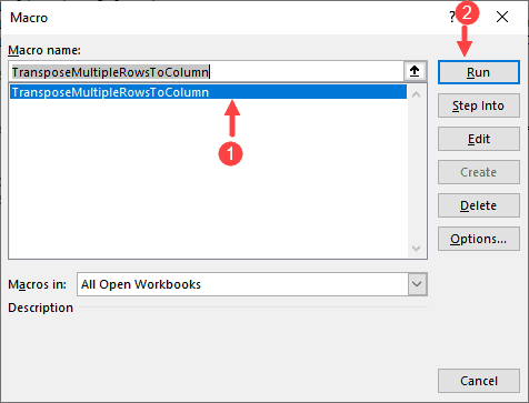
5. Press “Alt + F8” to open the “Macro” dialog box, select the “TransposeMultipleRowsToColumn” macro on the “Macro name” list box and click “Run.”

The “Transpose Multiple Rows to Column” dialog box is displayed.

6. Drag to select the range to transpose. The range is entered onto the “Source Ranges” field of the “Transpose Multiple Rows to Column” dialog box. Click “OK.”

The “Transpose Multiple Rows to Column” dialog box is displayed again.

7. Select a blank cell on the worksheet (in this example, we have selected cell E2). The cell reference is entered onto the “Convert to (single cell)” field. Click “OK.”

Immediately, the multiple rows of data are transposed into a single column, as shown below:

Explanation of the VBA Code

This macro transposes data from rows into a single column. It prompts the user to select the range to transpose and the cell where the transposed data should begin.

It loops through each row of the selected range, transposing and pasting it into the destination range, and moves down the column by the number of cells that were in the original row.

Screen updating is disabled during the operation to speed up the process and then re-enabled afterward.

This tutorial showed four techniques for transposing multiple rows in Excel into one column. We hope you found the tutorial helpful.

Other Excel articles you may also like:

• Row vs Column in Excel – What’s the Difference?
• Microsoft Excel Terminology (Glossary)
• Transpose in Excel (Shortcuts)
• How to Split One Column into Multiple Columns in Excel
• How to Select Multiple Rows in Excel?