Excel has some powerful Filter options (with inbuilt filter, advanced filter, and now the FILTER function in Office 365).
But none of these options actually filter as you type (i.e., show you the filtered data dynamically while you’re typing).
Something as shown below:
Although there is no inbuilt filter feature to do this, you can easily create something like this in Excel.
In this Excel tutorial, I will show you two simple ways to filter as you type in Excel.
The first method will be using the FILTER function (which you can access only in Office 365, now called Microsoft 365) and the other method would be by using a simple VBA code.
So let’s get started!
Filter as You Type (Using FILTER Function, No VBA Needed)
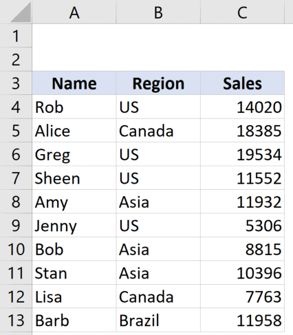
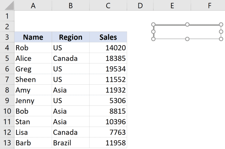
Suppose you have a dataset as shown below and you want to quickly filter data based on the region as you’re typing in a search box (which we will insert in the worksheet).
The first step is to insert a text box where you can type a text string and it will use it to filter the data (while you’re typing).
Below are the steps to insert the text box:
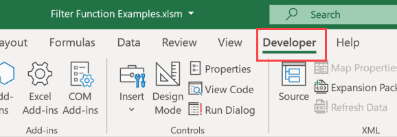
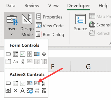
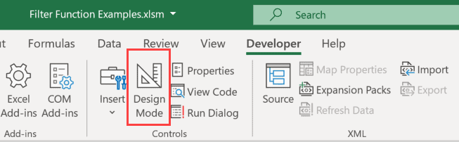
- Click the Developer tab.
- In the Control group, click on Insert.
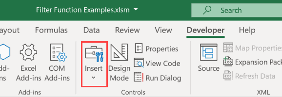
- Click on the Text Box icon in the ActiveX Controls
- Place the cursor anywhere in the worksheet, click and drag. This will insert a text box in the worksheet. You can place this text box wherever you want and can also resize it.
In case you don’t see the Developer tab in the ribbon (in Step 1), right-click on any of the tabs and click on ‘Customize the Ribbon’. In the Excel Options dialog box that opens, check the Developer option in the right pane and click OK. This will make the Developer tab visible in the ribbon.
Now that we have the text box in the worksheet, the next step is to connect it to a cell in the worksheet so that when you type anything in the worksheet, it will also automatically be entered in a cell.
This will allow us to use the value in the cell to filter the data.
Below are the steps to link the text box to a cell:
- Double-click on the text box. This will open the VB Editor.
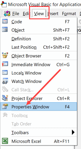
- Click the View option in the menu and then click on Properties Window. This will show the Properties Window Pane for the text box.
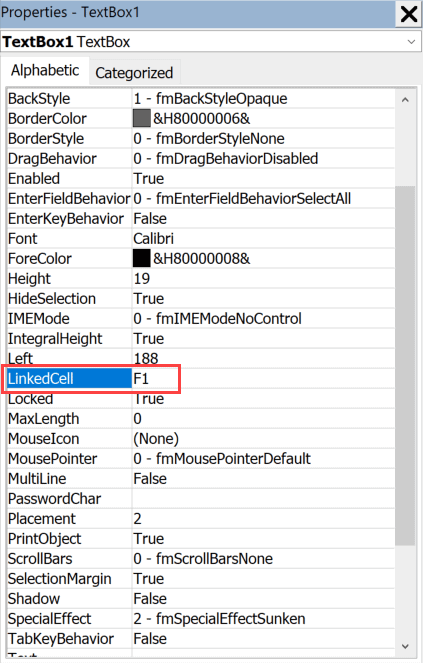
- In the properties window, come to the Linked Cell option and enter F1. This is the cell that we are connecting to the text box
- Close the VB Editor
- Go to the Developer tab, and click on the Design mode. You will notice that it turns from dark gray to light gray (indicating that it’s not enabled now).
Now, when you enter any text in the text box, you will notice that it appears in cell E1 in real-time (as you’re typing)
Now that we have linked the text box to a cell, the last step is to filter the data based on the value in the text box (which in turn would be the value in cell E1)
For this, we need to enter the FILTER formula in cell E4, so that results are filtered and shown there.
Below is the formula that will now filter the results as soon you can enter anything in the text box:
=FILTER(A4:C13,ISNUMBER(SEARCH(E1,B4:B13)))
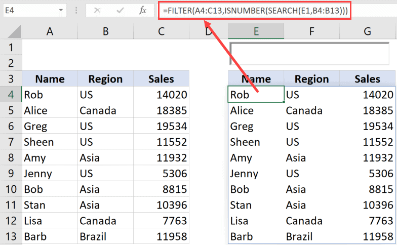
The above formula uses the FILTER function with the array as the original dataset and the condition uses the SEARCH formula.
The SEARCH formula checks whether the value entered in the text box (which also automatically gets entered in cell E1) is there in the cells in column B or not. All the cells that have the text will return a number and those that don’t will return the #VALUE! error.
The ISNUMBER function is used to get TRUE if there is a match and the cell returns a number, and FALSE is it returns the error.
Based on this condition, the data is filtered as you type.
Note that this formula checks whether the text string entered in the text box appears in the cells in column B or not. For example, if you enter ‘a’ in the text box, it would return all the records for Canada, Asia, and Brazil.
The position of the text string in the cells in column B is not checked.
In case you want to have the text string (that you enter in the search box) at the beginning only, you can use the below formula instead:
=FILTER(A4:C13,LEFT(B4:B13,LEN(E1))=E1)
Now when you enter A in the search box, it will only give you records for Asia.
Also read: VBA Macro Codes to Filter Data In Excel
Filter as You Type (Using VBA)
If you’re not using Office 365 and don’t have access to the FILTER function, you can still create the ‘filter as you type’ search box in Excel.
This can be done by using a really simple VBA code mentioned below:
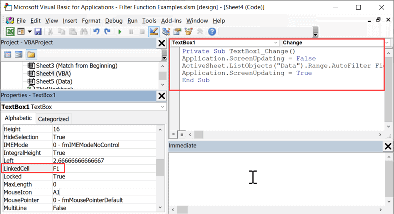
Private Sub TextBox1_Change()
Application.ScreenUpdating = False
ActiveSheet.ListObjects("Data").Range.AutoFilter Field:=2, Criteria1:= "*" & [A1] & "*", Operator:=xlFilterValues
Application.ScreenUpdating = True
End Sub
To use this code, you will have to first insert the text box in the worksheet and then add this code for the text box.
But the first step is to convert the data into an Excel table. While you can use this code without converting the data into an Excel table, it will be easier when the data is in Table as it becomes easier to refer to in the VBA code.
Below are the steps to convert the data into an Excel table:
- Select any cell in the dataset
- Hold the Control key and press the T key (or Command + T if you’re using a Mac).
- In the Create Table dialog box that opens, check whether the range is correct or not.
- Click Ok
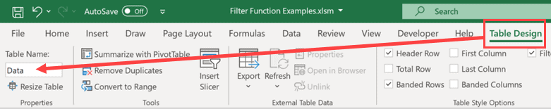
- Select any cell in the Excel Table
- Click on the ‘Table Design’ tab
- Change the name of the table to Data. You can use any name you want, but make sure to use the same one in the VBA code as well.
Below are the steps to insert the text box in the worksheet:
- Click the Developer tab.
- In the Control group, click on Insert.
- Click on the Text Box icon in the ActiveX Controls
- Place the cursor anywhere in the worksheet, click and drag. This will insert a text box in the worksheet. You can place this text box wherever you want and can also resize it.
Now that you have the text box in the sheet, you need to connect to a cell and then add the VBA code to the text box code window.
Below are the steps to do this:
- Double-click on the text box. This will open the VB Editor.
- Click the View option in the menu and then click on Properties Window. This will show the Properties Window Pane for the text box.
- In the properties window, come to the Linked Cell option and enter F1. This is the cell that we are connecting to the text box
- In the code window of the Text Box, copy and paste the above VBA code
- Close the VB Editor
- Go to the Developer tab, and click on the Design mode. You will notice that it turns from dark gray to light gray (indicating that it’s not enabled now).
Now you have a text box that is linked to a cell and this cell is used in the VBA code to filter the data.
When you enter any text in the text box, you will see that it filters the table in real tile (filter the data as you type in the text box).
Note: Since the VBA code is executed every time you enter a character in the text box, this method could make your workbook slightly slow in case you have a large data set. In such a case, instead of using the code in the text box code window, you can use it in a regular module and then assign it to a button. That way, you can first type the text in the text box and then click on the button to filter the data.
So these are two methods you can use to create a dynamic filter in Excel (filter data as you type).
Hope you found this tutorial useful!
You may also like the following Excel tutorials:
- How to Clear Contents in Excel without Deleting Formulas
- How to Clear Filter in Excel? Shortcut!
- 100 Useful Excel VBA Macro Codes Examples
- How to Hide Rows based on Cell Value in Excel
- How to Unhide All Rows in Excel with VBA
- How to Delete a Sheet in Excel Using VBA
- How to Select Alternate Columns in Excel (or every Nth Column)
- How to Select Every Other Cell in Excel (Or Every Nth Cell)
- How to Paste in a Filtered Column Skipping the Hidden Cells
- Filter Strikethrough in Excel
Thank you a lot. Wish you all the best.
One note, because we linked the text box to cell F1, so the VBA code suppose
Criteria1:= “*” & [F1] & “*”
instead of
Criteria1:= “*” & [A1] & “*”
is it correct?
Hi Thanks for the wonderful presentation.
I was wondering if
Range.AutoFilter Field:=2
can be modified to any field ?