How to Round to Significant Figures in Excel

Rounding to significant figures in Excel lets you report lab or science results to a consistent precision, even when your numbers have very different sizes.

Counting starts at the first nonzero digit, so your three significant figures could mean 12.5 or 0.00579.

Rounding both to the same number of decimal places won’t work. You need a formula that adjusts for each number’s size.

I’ll show you formulas that round the actual values and formatting that displays three significant figures while keeping the original readings.

Method #1: Using ROUND With LOG10

I recommend ROUND with LOG10 for most people because you get rounded numbers you can use in further calculations.

ROUND rounds to the number of decimal places you specify, but one fixed setting won’t work for readings of very different sizes.

Adding LOG10 lets you work out where the third significant digit falls in each number.

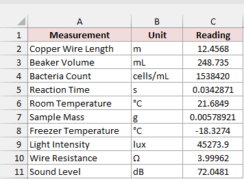
Below I have a dataset of lab readings in column C, ranging from tiny fractions to over a million. I want each rounded to three significant figures.

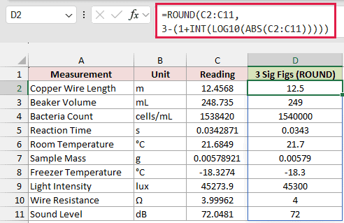
Here is the formula you can enter in D2.

=ROUND(C2:C11,3-(1+INT(LOG10(ABS(C2:C11)))))

You only enter it once in Excel 365 or Excel 2021 because it spills down the column automatically, filling D2:D11 with the rounded readings.

How does this formula work?

ABS returns 18.3274 for the Freezer Temperature reading of -18.3274, removing the minus sign. I need that because LOG10 can’t take a negative number.

LOG10 measures the number’s size in powers of 10. For the Bacteria Count reading of 1538420, it returns approximately 6.187.

INT then rounds that result down to the next lower whole number, giving 6.

Adding 1 counts the digits left of the decimal point. For 1538420, that’s 1+6, or seven digits.

I subtract those seven digits from the three significant figures I want. That leaves -4 for ROUND’s second argument, which tells it where to round.

A negative second argument tells ROUND to round left of the decimal point. Here, ROUND(1538420,-4) returns 1540000, the nearest ten thousand.

LOG10 of the Sample Mass reading, 0.00578921, is approximately -2.237. INT rounds this down to -3, not -2.

Here, -2 is the result of 1+(-3). For this tiny fraction, that negative result accounts for the zeros before the first significant digit.

The calculation 3-(-2) gives five decimal places, so ROUND(0.00578921,5) returns 0.00579.

ROUND still uses the original reading, so your Freezer Temperature reading keeps its negative sign and rounds to -18.3.

You can change the 3 in the formula to get a different number of significant figures.

You’ll see 4 and 72 instead of 4.00 and 72.0. Trailing zeros are zeros at the end that numeric results drop. Method #3 keeps them.

If you’re using Excel 2019 or earlier, you can enter this single-cell formula in D2 and copy it down.

=ROUND(C2,3-(1+INT(LOG10(ABS(C2)))))

Note: You’ll get #NUM! for a zero reading because LOG10 can’t take 0. You can use IF to return 0 for those readings instead: =IF(C2:C11=0,0,ROUND(C2:C11,3-(1+INT(LOG10(ABS(C2:C11))))))

Method #2: Using the TEXT Function

You can get the same rounded numbers with a shorter formula that also handles zero.

Writing 1540000 as 1.54E+6 means 1.54 multiplied by 10 to the sixth power. That’s scientific notation.

I use TEXT to produce that notation with three significant figures, then VALUE to turn the text back into a number.

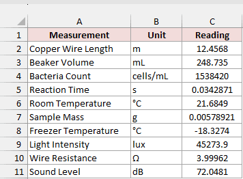
Below I have lab readings of different sizes in column C. I want to round each reading to three significant figures and keep the results numeric.

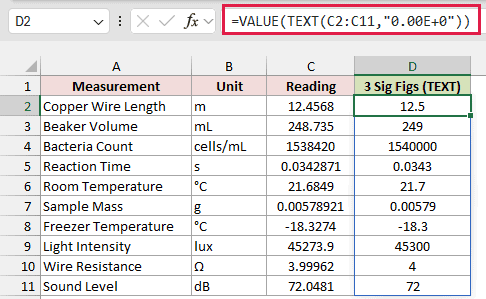
Enter this shorter formula in D2.

=VALUE(TEXT(C2:C11,"0.00E+0"))

You’ll get the rounded readings in D2:D11 as the formula spills down the column automatically. For example, you’ll get 12.5 and 1540000.

How does this formula work?

The scientific number format “0.00E+0” tells TEXT to keep one digit before the decimal point and two after it. That gives you three significant figures.

For Bacteria Count, the text “1.54E+6″ comes from TEXT(1538420,”0.00E+0”). VALUE converts it to the number 1540000.

You can use “0.0E+0” for two significant figures or “0.000E+0” for four. You need one zero per figure before the E.

Changing the precision means editing zeros inside the format code, rather than changing one number as you do in Method #1.

Method #3: Using the FIXED Function (Keeps Trailing Zeros)

You may need your lab report to show 4.00 rather than 4, so the reader can see all three significant figures.

I use FIXED for this because it returns text, which keeps those trailing zeros.

Below I have lab readings in column C that range from small fractions to large counts. I want three significant figures, including trailing zeros where needed.

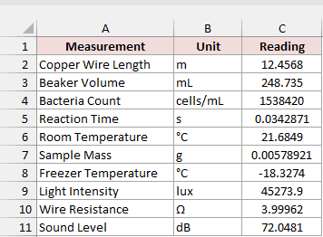
To keep those zeros, you can enter this formula in D2.

=FIXED(C2:C11,3-(1+INT(LOG10(ABS(C2:C11)))))

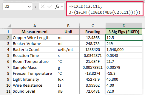
You’ll get text results as the formula spills down the column automatically into D2:D11. You’ll see 4.00 for Wire Resistance and 72.0 for Sound Level.

How does this formula work?

FIXED rounds each reading and returns text. It always shows the requested number of decimal places, even when they’re zeros.

The second argument works the same way as in Method #1. For Wire Resistance, it keeps two decimal places, so 3.99962 becomes 4.00.

For Sound Level, one decimal place turns 72.0481 into 72.0. You can now see the three significant figures in both results.

You’ll also see commas separating thousands, such as 1,540,000 and 45,300. You can add TRUE as FIXED’s third argument to remove them.

Left alignment tells you the results are text. SUM and AVERAGE ignore these text cells, so use a numeric method for further calculations.

A zero reading still returns #NUM! because the formula uses LOG10.

Method #4: Using a Custom LAMBDA Function

You can save yourself some typing if you round to significant figures often.

I use LAMBDA to build a function named SIGFIG, then call it like a built-in function. You need Excel for Microsoft 365 or Excel 2024.

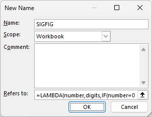
In the New Name dialog box used by Excel’s Name Manager, you can save a name for your formula.

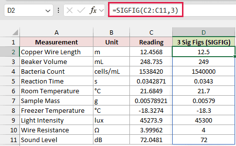
Below I have lab readings of very different sizes in column C. I want my SIGFIG function to round each one to three significant figures.

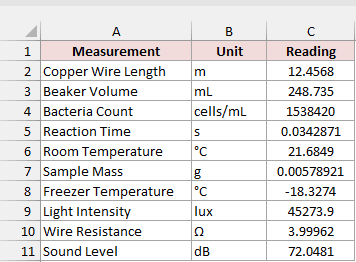
Here are the steps to create the SIGFIG function:

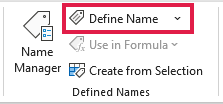
1. Go to the Formulas tab and click Define Name in the Defined Names group.

2. In the New Name dialog box, type SIGFIG in the Name field.

3. In the Refers to field, enter the LAMBDA formula below.

=LAMBDA(number,digits,IF(number=0,0,ROUND(number,digits-(1+INT(LOG10(ABS(number)))))))

4. Click OK.

Now you can use it like any other function by entering this formula in D2.

=SIGFIG(C2:C11,3)

You’ll get the rounded readings in D2:D11 as the formula spills down the column automatically, just as you did with Method #1.

How does this formula work?

The two inputs are number and digits. You pass the readings as the first argument and the number of significant figures as the second.

IF returns 0 for a zero reading, avoiding #NUM!. For other readings, I’ve used Method #1’s formula with those inputs in place.

You can use SIGFIG only in the workbook where you created it. To use it elsewhere, you need to create it in that workbook too.

Method #5: Using the Scientific Number Format

You can also show three significant figures without entering a formula.

I use the Scientific number format for display or printing. You change how the readings look while keeping the original values for calculations.

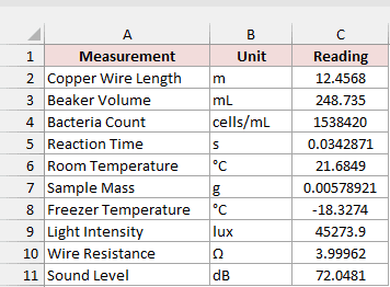
Below I have lab readings of different sizes in column C. I want to display each with three significant figures while keeping the full reading.

You can apply the Scientific number format with these steps:

1. Select the readings in C2:C11.

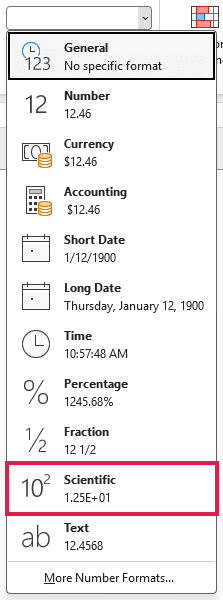
2. On the Home tab, open the Number Format drop-down in the Number group and choose Scientific.

You’ll now see each reading with three significant figures, such as 1.25E+01 for Copper Wire Length and 1.54E+06 for Bacteria Count.

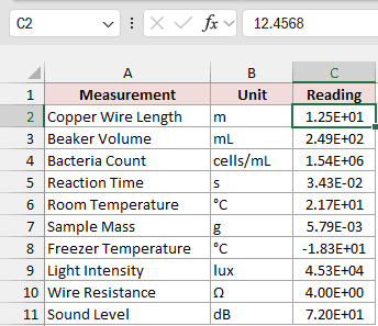
Scientific shows two decimal places by default. Together with the digit before the decimal point, that gives you three significant figures.

You can use Increase Decimal or Decrease Decimal on the Home tab to adjust the precision. Each extra decimal place adds one significant figure.

If you select C2, you’ll still see 12.4568 in the formula bar. Any formula referencing that cell uses the full value, even though you see 1.25E+01.

Additional Notes About Rounding to Significant Figures in Excel

Keep these differences in mind when you report or calculate with rounded readings:

• Methods #1-#4 give you new rounded values. Method #5 changes only the display, so calculations still use the original readings.
• Left alignment helps you spot FIXED’s text results. SUM and AVERAGE ignore those cells, so use numeric results when you need totals or averages.
• A number like 1540000 doesn’t tell you whether three or seven figures are significant. Showing 1.54E+06 in scientific notation makes the intended precision clear.
• The range formulas spill automatically in Excel 365 or Excel 2021. In older versions, use a single-cell formula and copy it down. LAMBDA needs Excel for Microsoft 365 or Excel 2024.

Frequently Asked Questions

Here are a few questions you might have about precision and rounding direction.

How do I round to 2 or 4 significant figures in Excel?

Replace the 3 in the ROUND formula with 2 or 4. For 12.4568, you’ll get 12 or 12.46, respectively.

The TEXT format needs “0.0E+0” for two significant figures or “0.000E+0” for four. You’ll get the same results after VALUE converts the text.

How do I always round up or down to significant figures?

Replace ROUND with ROUNDUP or ROUNDDOWN and keep the same second argument. ROUNDUP rounds away from zero, while ROUNDDOWN rounds toward zero.

For the Beaker Volume reading of 248.735, you’ll get 249 with ROUNDUP and 248 with ROUNDDOWN at three significant figures.

How many significant figures does Excel store?

Excel stores at most 15 significant digits of precision for a number. Rounding to more significant figures won’t increase that precision.

Conclusion

I covered five ways to handle significant figures, including formulas that round the actual value and Scientific number format, which changes only the display.

For most people, I’d use ROUND with LOG10 to round to the number of significant figures you need.

I hope you found this article helpful.

Other Excel articles you may also like:

• How to Round to the Nearest Whole Number in Excel (5 Easy Ways)
• CEILING.MATH Function in Excel (5 Easy Examples)
• MROUND Function in Excel (6 Easy Examples)
• Round to the Nearest Tenth in Excel (Easy Formulas)
• How to Remove Decimals in Excel? (3 Easy Ways)
• Round Numbers in Excel Without Using Formula (4 Easy Ways)
• FLOOR.MATH Function in Excel (6 Easy Examples)