How to VLOOKUP From Another Sheet in Excel

VLOOKUP from another sheet is what you need when your prices or product details live on one tab and the rows you’re filling in live on another.

The lookup works exactly like a normal VLOOKUP. The only difference is the table_array argument.

It now has to name the other sheet (and sometimes the other workbook) before the range.

That reference is the tricky part. One missing apostrophe or exclamation mark, and you get an error instead of a price.

Letting Excel write the reference for you avoids most of those slips.

In this article, I’ll show you how to click your way to the formula, look up from a separate workbook, search two sheets with IFERROR, and use an Excel Table.

Method #1: Using a Range on Another Sheet

This is the method you’ll use most of the time. The lookup table sits on a different tab in the same workbook, and VLOOKUP points at it.

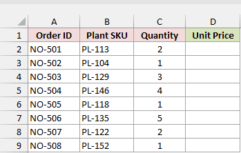
Below I have the Nursery Orders sheet. Each row has an order ID, a plant SKU, and a quantity.

I want column D to show the unit price for each SKU.

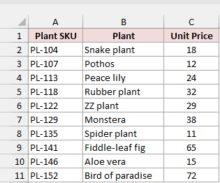
The prices are on a separate sheet called Plant Catalog. It has the SKU in column A, the plant name in column B, and the unit price in column C.

Here are the steps to pull the prices in by pointing and clicking:

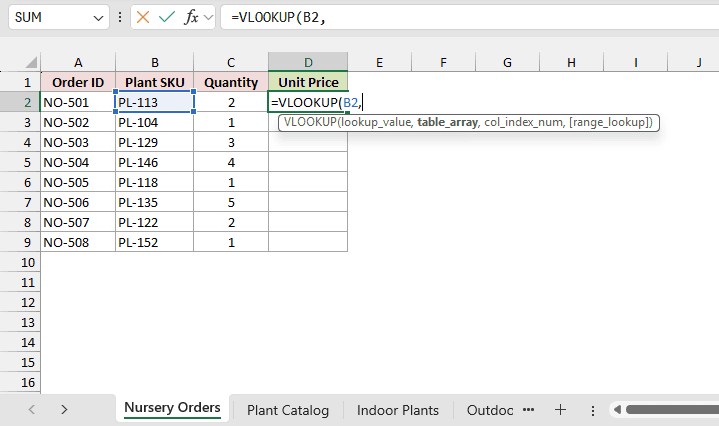
1. On the Nursery Orders sheet, select cell D2 and type =VLOOKUP(B2, (don’t press Enter yet).

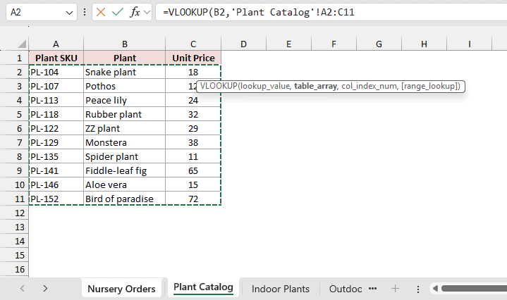
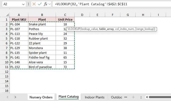
2. Click the Plant Catalog sheet tab and select the range A2:C11. Excel adds 'Plant Catalog'!A2:C11 to the formula for you.

3. Press F4 once. This turns the range into $A$2:$C$11, so it stays fixed when you copy the formula down.

4. Type ,3,FALSE) and press Enter. Excel takes you back to Nursery Orders. Then double-click the fill handle in D2 to copy the formula down to D9.

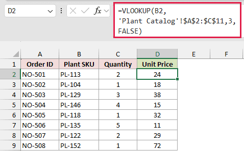
Here is the formula you end up with in D2:

=VLOOKUP(B2,'Plant Catalog'!$A$2:$C$11,3,FALSE)

How does this formula work?

B2 is the SKU I want to find. For order NO-501, that’s PL-113.

<code>’Plant Catalog’!$A$2:$C$11</code> tells VLOOKUP to search A2:C11 on the Plant Catalog sheet. The exclamation mark separates the sheet name from the range.

The apostrophes are there because the sheet name has a space in it. The dollar signs lock the range, so every copied formula still points at the full catalog.

The 3 returns the third column of that range (Unit Price), and FALSE asks for an exact match. For NO-501, the formula returns 24.

I’m using one formula per row here because it works in every Excel version. In Excel 2021 and later, <code>=VLOOKUP(B2:B9,’Plant Catalog’!$A$2:$C$11,3,FALSE)</code> in D2 spills all eight prices at once.

Note: Always keep FALSE at the end. Without it, VLOOKUP does an approximate match, and a SKU that isn’t in the catalog (like PL-150) quietly returns 15, the price of PL-146.

Method #2: Using a Range in Another Workbook

If your catalog lives in its own file, VLOOKUP can read from that file too. This is handy when several workbooks share one price list.

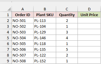
Below I have the same Nursery Orders sheet with an empty Unit Price column.

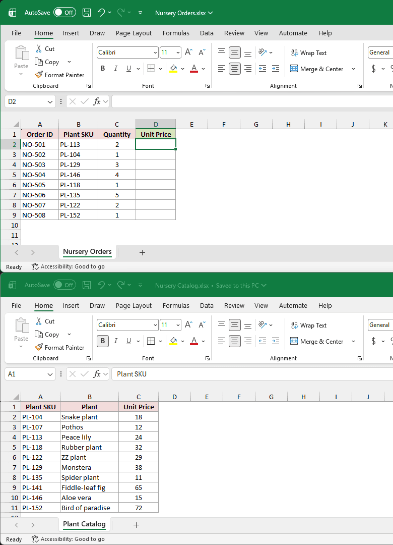
This time, the prices are in a separate workbook called Nursery Catalog.xlsx, on a sheet named Plant Catalog.

To follow along with the download, right-click the Plant Catalog tab and choose Move or Copy. Pick (new book) under To book, check Create a copy, and click OK.

Save that new workbook as Nursery Catalog.xlsx. You now have two files: the download with Nursery Orders, and the catalog workbook.

Here are the steps to look up the prices from the other workbook:

1. Open both workbooks: the one with Nursery Orders and Nursery Catalog.xlsx.

2. In the orders workbook, select D2 on the Nursery Orders sheet and type =VLOOKUP(B2, (don’t press Enter).

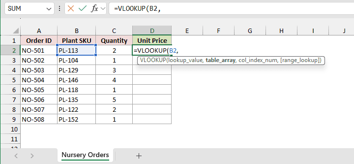
3. Switch to the Nursery Catalog.xlsx window (click it on the taskbar) and select A2:C11 on its Plant Catalog sheet. Excel adds the workbook name and locks the range with dollar signs on its own.

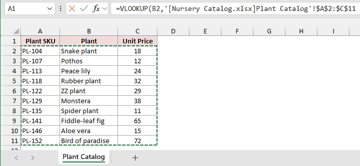
4. Type ,3,FALSE), press Enter, and fill the formula down to D9.

Here is the formula Excel builds in D2 while both files are open:

=VLOOKUP(B2,'[Nursery Catalog.xlsx]Plant Catalog'!$A$2:$C$11,3,FALSE)

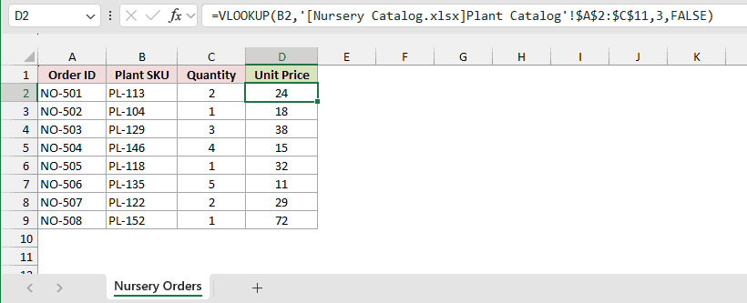
How does this formula work?

It’s the same lookup as Method #1. The new part is <code>[Nursery Catalog.xlsx]</code>, the workbook name in square brackets, which sits right before the sheet name.

The apostrophes now wrap both the workbook and sheet names. The result is the same too: 24 for order NO-501.

What Happens When the Source Workbook Is Closed

Close Nursery Catalog.xlsx and look at D2 again. Excel now shows the full folder path, so it knows where to find the file:

=VLOOKUP(B2,'C:\Steve\[Nursery Catalog.xlsx]Plant Catalog'!$A$2:$C$11,3,FALSE)

The formula still returns 24. Excel keeps the values from the last time the link updated, so the catalog doesn’t have to stay open.

Your path will match wherever you saved the catalog. You don’t type it yourself. Excel writes it when you close the source file.

When you reopen the orders workbook later, Excel may show a security warning that automatic update of links has been disabled. Click Enable Content to pull in the latest prices.

To check or fix the link, go to Data > Workbook Links. If your version doesn’t have that button, use Data > Edit Links instead.

Note: If you move or rename Nursery Catalog.xlsx, the link breaks and the formula can’t refresh. Use Change source in Workbook Links (or Change Source in Edit Links) to point it at the file’s new location.

Method #3: Using IFERROR to Search Multiple Sheets

Sometimes the values you need are split across two or more sheets. VLOOKUP only searches one range, but you can chain a few of them together with the IFERROR function.

Below I have the Garden Orders sheet. It has nine orders, and the SKUs come from two different price lists.

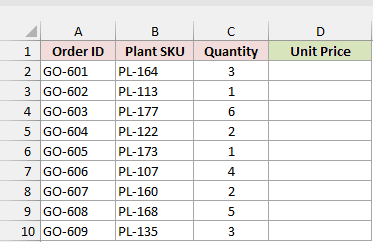
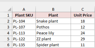
Indoor plants are on the Indoor Plants sheet, with the SKU in column A and the price in column C.

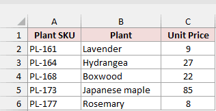
Outdoor plants are on the Outdoor Plants sheet, in the same layout. One order (GO-607) uses PL-160, which isn’t on either sheet.

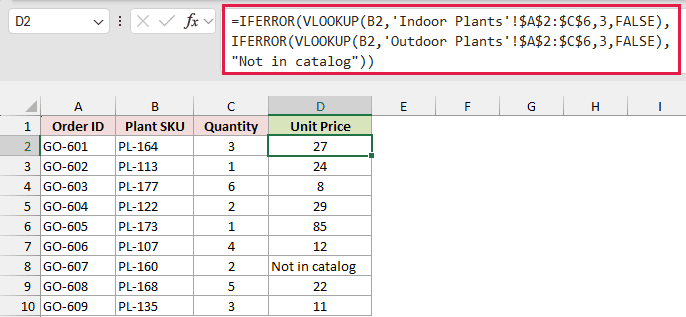
Here is the formula to enter in D2 and copy down to D10:

=IFERROR(VLOOKUP(B2,'Indoor Plants'!$A$2:$C$6,3,FALSE),IFERROR(VLOOKUP(B2,'Outdoor Plants'!$A$2:$C$6,3,FALSE),"Not in catalog"))

How does this formula work?

The first VLOOKUP searches the Indoor Plants sheet. If it finds the SKU, that price is the answer.

If it doesn’t, it returns #N/A, and the outer IFERROR moves on to the second VLOOKUP, which searches Outdoor Plants. That’s how GO-601 (PL-164) gets 27.

If the SKU isn’t on either sheet, the inner IFERROR returns “Not in catalog” instead of an error. You can see that for GO-607.

If you have a third sheet, add one more IFERROR(VLOOKUP(…)) layer before the “Not in catalog” text.

With lots of sheets that share a layout, the INDIRECT function can build the sheet reference from a name typed in a cell.

Keep in mind that INDIRECT won’t update if someone renames a sheet.

Method #4: Using an Excel Table or Named Range

Here’s another way to set this up, and it’s my favorite when the lookup list keeps growing. Instead of a sheet name and a range, the formula uses a name.

Below I have the Price List sheet with the same ten plants. Right now it’s a plain range.

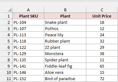
Here are the steps to turn it into a Table and look up from it:

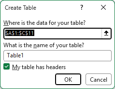
1. Select any cell in the price list, press Ctrl + T, make sure My table has headers is checked, and click OK. If your dialog also has a table name box, you can type PlantCatalog there and skip the next step.

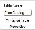
2. On the Table Design tab, type PlantCatalog in the Table Name box and press Enter.

3. Go to the Table Orders sheet, enter the formula below in D2, and copy it down.

=VLOOKUP(B2,PlantCatalog,3,FALSE)

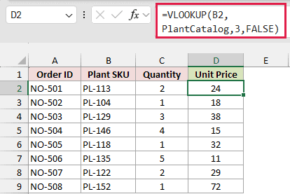
How does this formula work?

PlantCatalog is the Table’s name. In a formula, it means the Table’s data rows (A2:C11 right now, without the header).

There’s no sheet name, no apostrophes, and no dollar signs to worry about. The name works from any sheet in the workbook, and NO-501 still returns 24.

The real benefit shows up when the list changes.

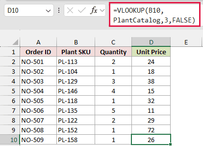
Below, I typed a new plant, Calathea (PL-158), in row 12 right under the Table. The Table grew to include it.

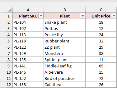
Now a new order for Calathea (NO-509) returns 26 on the Table Orders sheet. I didn’t have to touch the formula, because PlantCatalog already includes row 12.

Note: If you’d rather use a named range, select A2:C11 on the Plant Catalog sheet, type PlantPrices in the Name Box, and press Enter. Then use =VLOOKUP(B2,PlantPrices,3,FALSE). Unlike a Table, the name won’t grow with new rows.

Additional Notes About VLOOKUP From Another Sheet in Excel

• Renaming the source sheet is safe. Excel updates every formula that points to it. Deleting the sheet isn’t: every lookup turns into #REF!, and a sheet delete can’t be undone.
• #N/A usually means the value isn’t there in exactly the same form. A trailing space (“PL-113 “) or an ID stored as a number on one sheet and as text on the other is enough to break the match. TRIM fixes the space problem.
• A column number bigger than the range returns #REF!. With the three-column range used here, 4 fails.
• A whole-column range like <code>’Plant Catalog’!$A:$C</code> keeps working when rows are added, but a Table (Method #4) does the same job more neatly.
• To remove the dependence on another workbook, paste the results as values or break the links.

Frequently Asked Questions

Here are answers to a few common questions about using VLOOKUP across sheets.

Can I use XLOOKUP instead of VLOOKUP to get data from another sheet?

Yes, if you have Excel 2021, Excel 2024, or Microsoft 365. XLOOKUP takes the search column and the return column separately, so there’s no column number to count:

=XLOOKUP(B2,'Plant Catalog'!$A$2:$A$11,'Plant Catalog'!$C$2:$C$11)

For NO-501, this returns 24, the same as the VLOOKUP version.

How do I VLOOKUP multiple columns from another sheet?

Give VLOOKUP an array of column numbers. In Excel 2021 and later, this formula spills the plant name and the price into two cells (Peace lily and 24 for NO-501):

=VLOOKUP(B2,'Plant Catalog'!$A$2:$C$11,{2,3},FALSE)

What happens to my VLOOKUP if someone inserts a column in the other sheet?

The range expands to include the new column, but the 3 stays a 3. So the formula returns the wrong column, and Excel shows no error.

To avoid that, let MATCH find the column number from the header. This version still returns 24 after a column is inserted:

=VLOOKUP(B2,'Plant Catalog'!$A$2:$C$11,MATCH("Unit Price",'Plant Catalog'!$A$1:$C$1,0),FALSE)

Do I need apostrophes around the sheet name?

Only when the name has spaces, starts with a number, or contains most punctuation. A sheet called Catalog works as <code>Catalog!$A$2:$C$11</code>.

If you click the sheet tab while building the formula, Excel adds the apostrophes when they’re needed.

Conclusion

In this article, I showed you how to VLOOKUP from another sheet by pointing and clicking.

I also covered separate workbooks, two sheets at once with IFERROR, and an Excel Table.

For most lookups, Method #1 is all you need. If your list keeps growing, the Table version saves you from ever updating the range.

I hope you found this article helpful.

Other Excel articles you may also like:

• VLOOKUP Not Working (7 Possible Reasons + Fix)
• How to Use VLOOKUP with Multiple Criteria in Excel
• XLOOKUP vs VLOOKUP in Excel
• How to Reference a Cell on Another Sheet in Excel
• Using VLOOKUP Approximate Match in Excel (Examples)
• How to Link Cells in Excel (Same Worksheet, Between Worksheets/Workbooks)
• IFNA Function in Excel