HYPERLINK Function in Excel (5 Easy Examples)

If you want to turn a cell into a clickable link in Excel, the HYPERLINK function is the cleanest way to do it.

HYPERLINK does not spill across cells like newer dynamic array functions, so you fill it down or pair it with a lookup.

In this article, I’ll show you how to use the HYPERLINK function with five practical examples.

Table of Contents

HYPERLINK Function Syntax in Excel

The HYPERLINK function builds a clickable jump from a cell to a destination.

=HYPERLINK(link_location, [friendly_name])

link_location (required): the path to jump to. Can be a web URL, a mailto: email, a file path, or a cell or named range inside the workbook (prefix with #).
friendly_name (optional): the text that shows in the cell. If you skip this, the cell displays the raw link_location instead.

When to Use HYPERLINK Function

Turn a column of URLs into clickable links without typing each one by hand.
Build clickable email links from a contact list.
Create a clickable table of contents that jumps to other parts of your workbook.
Combine with VLOOKUP, XLOOKUP, or INDEX/MATCH to return a clickable lookup result.
Generate search-engine query links (Google, YouTube, Amazon) from a list of terms.

Example 1: Make Cell Text Clickable Web Links

Let’s start with a simple example. You have a list of websites with their URLs in two columns, and you want a third column that shows each site name as a clickable link.

Below is the dataset. Column A has the site name and column B has the URL.

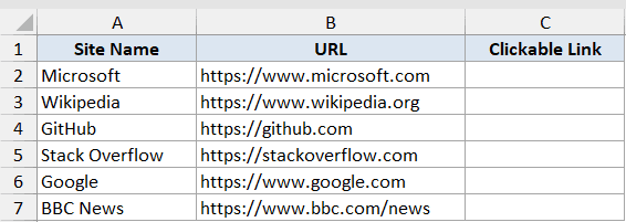
Hyperlink Function Dataset Example 1 showing an Excel table with columns for Site Name, URL, and Clickable Link

We want column C to display the site name from column A, but clicking the cell should open the URL in column B.

Here is the formula:

=HYPERLINK(B2, A2)

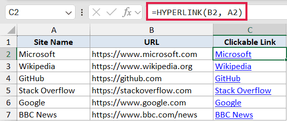
Excel formula bar showing =HYPERLINK(B2, A2) to create clickable links in column C based on site names and URLs

Here, link_location is B2 (the URL) and friendly_name is A2 (the site name). Excel formats the cell as a blue underlined link, and clicking it opens the URL in your default browser.

Fill the formula down column C and every row gets its own clickable link, tied to whatever URL sits in column B. If you ever change a URL, the link in column C updates automatically.

Pro tip: to select the cell without triggering the link, click and hold until the cursor turns into a plus sign, then release. Arrow keys also work without firing the link.

Example 2: Create Clickable Email Links with mailto

Here’s another practical scenario. You have a contact list with names and emails, and you want a third column that opens a fresh email draft when clicked.

Below is the dataset. Column A has the contact name and column B has the email address.

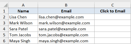
Hyperlink Function Dataset Example 2: Excel table with columns for Name, Email, and a blank Click to Email column

We want column C to display “Email <name>” as a clickable link that opens the default email client addressed to that person.

Here is the formula:

=HYPERLINK("mailto:"&B2, "Email "&A2)

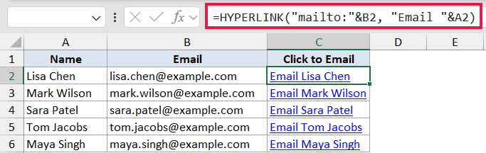
Excel formula bar showing HYPERLINK function with mailto argument to create clickable email links in a spreadsheet

The mailto: prefix tells the operating system to open the default email client instead of a browser. We concatenate it with the email in B2 using &, and build the display text by joining “Email ” with the name in A2.

A bare email address by itself won’t create a working email link. The mailto: prefix is required.

You can also pre-fill a subject line and body by extending the link:

=HYPERLINK("mailto:"&B2&"?subject=Quick%20Question&body=Hi%20"&A2, "Email "&A2)

The %20 is the URL-encoded space character. Use %0D%0A for a line break in the body.

Example 3: Jump to a Specific Cell with the # Prefix

Let’s step it up. HYPERLINK can also navigate within your own workbook, which is the basis for clickable tables of contents and quick-nav menus. The key is the # prefix.

Below is the dataset. Column A has a section name, column B has the target cell address.

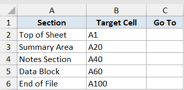
Hyperlink Function Dataset Example 3 showing an Excel table with columns for Section, Target Cell, and Go To links

We want column C to be a clickable label that jumps to the target cell on the current sheet when clicked.

Here is the formula:

=HYPERLINK("#"&B2, A2)

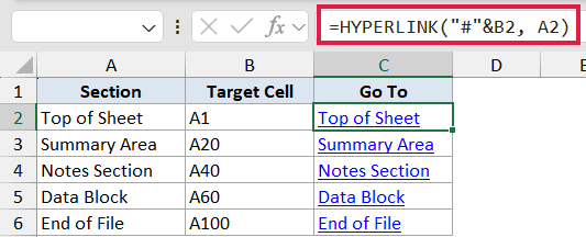
Excel formula bar showing =HYPERLINK("#"&B2, A2) to create internal sheet links in column C

The # prefix tells HYPERLINK that the destination is inside the current workbook, not a web URL or a file path. The text after # can be a cell address, a named range, or a sheet-qualified address like Sheet2!A1.

To jump to a cell on a different sheet, use "#Sheet2!A1". If the sheet name has a space, wrap it in single quotes: "#'Sales Data'!A1". To jump to a named range, use the name directly after the #, like "#TaxRate".

This pattern is the foundation of clickable navigation in Excel. You can build a small nav table at the top of a sheet, paste this formula in, and you have a working table of contents in under a minute.

Common mistake: people write =HYPERLINK("Sheet2!A1", "Jump") and wonder why it does not work. The # prefix is required for in-workbook jumps.

Example 4: Build a Clickable Link from a Lookup

Here’s the pattern I use most. You can combine HYPERLINK with XLOOKUP (or VLOOKUP) to return a clickable link based on whatever the user has selected.

Below is the dataset. The lookup table in columns A and B has site names and their URLs. Cell D2 has the currently selected site name, and we want E2 to show that name as a clickable link to the matching URL.

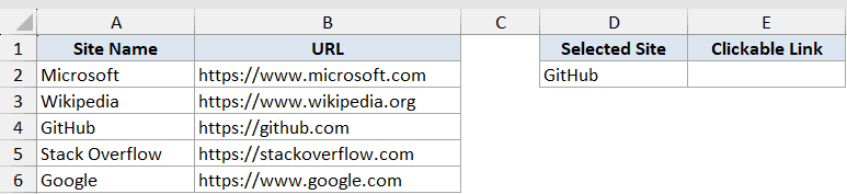
Hyperlink Function Dataset Example 4 showing a table of site names and URLs with a selected site field for linking

Here is the formula:

=HYPERLINK(XLOOKUP(D2,A2:A6,B2:B6), D2)

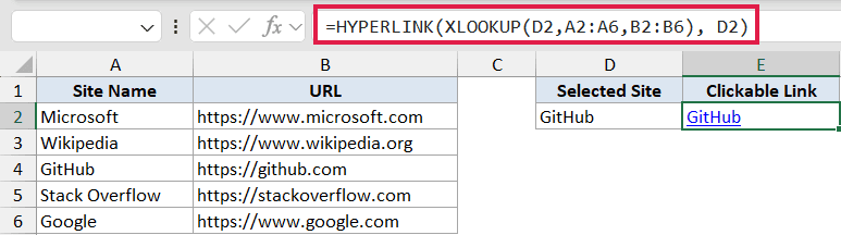
Excel formula bar showing HYPERLINK with XLOOKUP to create a dynamic clickable link based on a selected site name

How this formula works:

XLOOKUP(D2,A2:A6,B2:B6) looks up the value in D2 against column A and returns the matching URL from column B.
That URL is fed into HYPERLINK as link_location.
D2 is also used as friendly_name, so the cell displays the selected site name.
Change the value in D2 (or wire D2 to a data validation dropdown), and the clickable link updates instantly.

If you are on an older version of Excel without XLOOKUP, you can swap in VLOOKUP:

=HYPERLINK(VLOOKUP(D2, A2:B6, 2, FALSE), D2)

This is the pattern behind dashboard navigation widgets, “open the document for this client” buttons, and anything else where the link target depends on a selection.

Example 5: Build a Google Search Link from a Cell

Here is a fun one. You can build a clickable Google search link from any cell value, which is handy when you’re triaging a list of items and want to look each one up quickly.

Below is the dataset. Column A has a list of search terms.

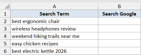
Excel dataset with Search Term in column A and empty Search Google cells in column B for HYPERLINK function example

We want column B to be a clickable Google search link for whatever is in column A.

Here is the formula:

=HYPERLINK("https://www.google.com/search?q="&A2, "Search Google for "&A2)

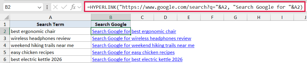
Excel formula bar showing a HYPERLINK function that dynamically creates Google search links based on cell A2 content

The https://www.google.com/search?q= part is the URL prefix Google uses for search queries. We concatenate the search term from A2, and the display text is built by joining “Search Google for ” with the term in A2.

If your search terms have spaces, you don’t need to URL-encode them yourself. Most browsers handle that automatically when the link opens.

The same pattern works for any site that accepts a URL-based search query. A few common ones:

YouTube: https://www.youtube.com/results?search_query=
Amazon: https://www.amazon.com/s?k=
Wikipedia: https://en.wikipedia.org/wiki/Special:Search?search=

Tips & Common Mistakes

The # prefix is required for in-workbook jumps. =HYPERLINK("Sheet2!A1", "Go") does not work. You need =HYPERLINK("#Sheet2!A1", "Go"). Sheet names with spaces need single quotes: "#'Sales Data'!A1".

HYPERLINK does not spill. Even on Excel 365, feeding HYPERLINK a range as link_location does not produce one clickable link per cell. Fill the formula down instead, or wrap each call in a MAP + LAMBDA workaround if you really need a single-formula version.

HYPERLINK is a formula, not a pasted hyperlink. The Insert > Hyperlink dialog (Ctrl+K) creates a static hyperlink attached to the cell. HYPERLINK creates a recalculating formula link. If you use VBA to iterate Worksheets.Hyperlinks, formula-based links won’t be in that collection.

The link_location has a 255-character limit. Anything longer returns #VALUE!. For very long URLs, run them through a URL shortener first.

Excel for the Web only supports web URLs. Local file paths and UNC network paths won’t navigate in the browser version.

Invalid links don’t error until you click them. The cell shows the formatted link as normal, and the error only pops up after the click. This makes broken hyperlinks easy to ship by accident, so double-check destinations before sharing the workbook.

To select a cell with HYPERLINK without triggering it, click and hold until the cursor becomes a plus sign, then release. Or navigate to it using the arrow keys.

HYPERLINK looks simple on the surface, but it ends up in a lot of useful places: clickable tables of contents, dynamic email lists, dashboard navigation, and lookup-driven links. The # prefix and & concatenation are the two pieces of glue you’ll keep coming back to.

Once you have the syntax down, the lookup-then-link pattern in Example 4 is the one most people reuse. Wire it to a data validation dropdown and you have a one-cell interactive nav widget for your workbook.

List of All Excel Functions