How to Remove Hyperlinks in Excel (Easy Step-by-Step)

Working with a spreadsheet full of hyperlinks can be quite frustrating.

Unless otherwise specified, Excel usually recognizes the formats of email addresses and URLs and automatically converts them to hyperlinks.

While this is helpful most of the time, it can also be a source of frustration.

In this tutorial, I will show you how to remove hyperlinks in Excel in a few clicks.

Table of Contents

Issues when Working with Hyperlinks in Excel

When you have some hyperlinks in your worksheet, you may feel some level of frustration dealing with it (at least I do).

Below are some of the issues you can face when you have hyperlinks in your workbook:

It’s difficult to select, copy, and delete cells containing hyperlinks. This is because when you click on the cell, Excel opens up your default browser and directly takes you to that link. This can feel more like unsolicited assistance and waste a lot of time. There is one way around this though. You can click on the cell and hold your mouse button till the pointer turns into a plus symbol. But this slows you down and is not helpful at all when you’re trying to get important work done.
Say you find an error in the URL of a website in one of the cells. To change or correct it, you need to double click the contents of the cell. This becomes really difficult when Excel marks the contents as a hyperlink.
If Excel sees any content that looks like a URL, email address, or file location, it automatically converts it into a hyperlink, even if that link doesn’t actually exist. This could mislead someone else going through your spreadsheet.

For all the above cases, the best solution would be to either remove the hyperlinks, so the cell contents behave and look like regular text, or to disable automatic hyperlink conversions altogether.

In this tutorial, we are going to look at how you can remove hyperlinks from a single cell, multiple cells, and a whole worksheet.

We will also show you how to disable Excel from automatically converting anything to a hyperlink.

Also read: Insert Hyperlink in Excel [Keyboard Shortcut]

Remove Hyperlink from a Single Cell

To remove a hyperlink from a single cell, right-click on the cell directly (don’t left-click to select it first).

Next, select “Remove Hyperlink” from the popup menu.

That’s all, your cell gets converted to a cell with regular text.

Bear in mind, though, that this removes any other formatting that had been applied to the cell too.

If you want to remove hyperlinks from a range of cells, here’s a quick, two-click method:

Select the range of cells containing the hyperlinks you want to remove.
Right-click on the selection and select “Remove Hyperlinks” from the dropdown menu.

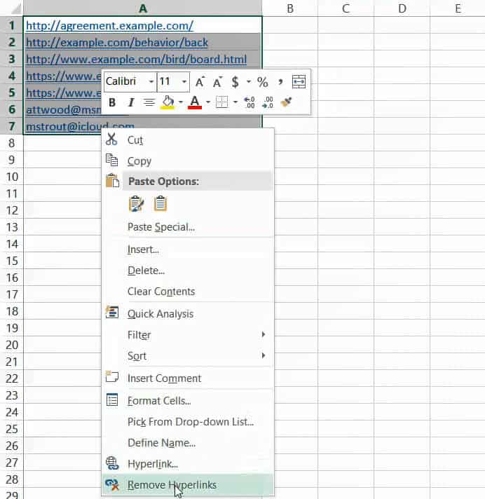
Again, this technique removes hyperlinks along with any formatting from the selected cells.

Also read: Excel Hyperlink Cannot Open the Specified File - Fix!

Remove all Hyperlinks from the Entire Worksheet

If you have hyperlinks in different areas of your spreadsheet, it’s quicker to just remove all the hyperlinks in the sheet at once.

Here’s how you can do this in just two clicks:

Select all the cells in your worksheet, either by clicking on the triangle on the top right corner of your sheet or pressing CTRL+A from the keyboard.
Right-click anywhere on your worksheet, and select “Remove Hyperlinks” from the dropdown menu.

This also removes all hyperlinks in the worksheet as well as any formatting done on the cells with links. Formatting of other cells, however, remains unchanged.

Clear Hyperlinks Without Changing Format Settings

If you would rather retain the formatting when removing hyperlinks, there’s another technique:

Select the cells you want to work on. You can select a single cell, group of cells, or the entire worksheet.
Under the Home tab, you will find the Clear option in the ‘Editing’ group. Click on it and select “Clear Hyperlinks” from the dropdown list.
When you do this, you will see a pink eraser icon. If you had selected a group of cells, the eraser should appear at the bottom right corner of your selection. If you had selected the entire worksheet, it should appear at the top right corner of your sheet.
Click on this eraser icon. You will see a drop-down list with two options:
- Clear Hyperlinks only
- Clear Hyperlinks and Formats
If you click on “Clear Hyperlinks only”, your hyperlinks will be removed, but formatting will remain intact. However, if you click on “Clear Hyperlinks and Formats”, it will remove both the hyperlinks as well as any formatting applied to those cells.

Note that hyperlinks automatically get a format where the text is blue with an underline. When you use the above method, it will remove the hyperlink, but it will not remove any formatting, including the blue text and underline.

So it may look as if there are hyperlinks in the cell, but it’s just the formatting.

Related: How to Extract URL from Hyperlinks in Excel (Using VBA Formula)

Remove hyperlinks with a VBA Macro

If you need to work with hyperlinks quite often and are comfortable using VB macros, you can create a simple macro script to do this..

To remove hyperlinks from a selection, here’s the code that you can use:

Sub RemoveSelectedHyperlinks()
Selection.Hyperlinks.Delete
End Sub

Follow these steps:

Select the range of cells for which you want to remove hyperlinks.
From the Developer Menu Ribbon, select Visual Basic.
Once your VBA window opens, Click Insert->Module. Now you can start coding. Type or copy-paste the above lines of code into the module window:
Run the macro by navigating to Developer->Macros->RemoveSelectedHyperlinks->Run or just clicking the button.
When you go back to your spreadsheet, you will find the selected all hyperlinks removed from the selection.

To remove hyperlinks from the entire sheet, you can use the following code:

Sub RemoveAllHyperlinks()
ActiveSheet.Hyperlinks.Delete
End Sub

Since you want to work on the entire sheet you don’t need to make any selections. Just make sure the sheet you want to apply the code on is the active sheet.

Follow these steps:

From the Developer Menu Ribbon, select Visual Basic.
Once your VBA window opens, Click Insert->Module. Now you can start coding. Type or copy-paste the above lines of code into the module window:
Run the macro by navigating to Developer->Macros-> RemoveAllHyperlinks ->Run or just clicking the button.
When you go back to your spreadsheet, you will find all hyperlinks removed from the entire sheet.

Once your VBScript is ready and working, you can link this to a macro button and add it to your quick access toolbar.

Here’s how to do this:

Click on the Customize Quick Access Toolbar dropdown. You will find it at the top of your Excel window.
Click on “More Commands”
This will open the Excel Options dialog box.
Click on the drop-down list below “Choose Commands From” and select the “Macros” option.
Select the name of the macro you created. In our case, it’s either ‘ThisWorkbook.RemoveSelectedHyperlinks’ or ‘ThisWorkbook.RemoveAllHyperlinks’.
Click on the Add>> button.
Click OK.

This will create a Quick Access macro button for you and place it on your Quick Access Toolbar, so whenever you click it, your macro can run and remove all your required hyperlinks.

In this way, you can get your hyperlinks removed even faster, with just one click.

Note: Running this macro will remove all your hyperlinks permanently, so you will not be able to reverse the changes even by using the Undo command.

Turn off Automatic Hyperlink Conversion for all Worksheets

Finally, if you don’t want to deal with automatic conversion to hyperlink altogether, you can turn off this feature. Here’s what you need to do:

Click on File->Options.
This will open the Excel Options dialog box. Select “Proofing” from the left sidebar.
Click the “AutoCorrect Options” button.
This will open the “AutoCorrect” dialog box. Click on the “AutoFormat As You Type” tab.
Uncheck the “Internet and Network Paths with Hyperlinks” checkbox.
Click OK to close the AutoCorrect dialog box.
Click OK to close the Excel Options dialog box.

This will take you back to your Excel sheet. Now if you type any URL, email address, or file location, Excel will retain it in regular text format, instead of converting it.

Note: At any point, if you want to convert the contents of a cell to a hyperlink, you can simply right-click the cell, select “Hyperlink” from the popup menu and then enter the address you want to link to.

Conclusion

In this tutorial, we showed you how to remove hyperlinks in Excel from a cell, a selection of cells, or an entire worksheet.

We also showed you how to get this done in one click by creating a macro. Finally, we showed you how you can prevent Excel from automatically converting any text to hyperlink unless you link them yourself.

Do let us know in the comments if you need any further clarification about anything explained in this tutorial.

Other Excel tutorials you may like: