If you want to project how much a savings account or investment will be worth in the future, the FV function is what you need. It handles both regular deposits and one-time lump sums, or a mix of both.
FV normally returns one number, but in Excel 365 you can feed a range into one argument and it spills a result for every input.
In this article, I’ll walk you through five practical examples that cover the most common ways to use it.
FV Function Syntax in Excel
Here is how the FV function is put together.
=FV(rate, nper, pmt, [pv], [type])
- rate is the interest rate per period. For monthly compounding, divide the annual rate by 12.
- nper is the total number of periods. For monthly contributions over several years, multiply years by 12.
- pmt is the regular payment each period, entered as a negative number because it is money going out.
- [pv] is an optional lump sum you already have. Also entered as a negative number. Skip it with a double comma if there is none. See the PV function if you need to work in the opposite direction.
- [type] is optional. Use 0 for payments at the end of each period (the default) or 1 for payments at the beginning.
When to Use FV Function
Here are some situations where FV is the right tool.
- Project the future balance of a savings account when you make regular monthly deposits.
- Find out how much a one-time investment will grow over time at a fixed rate, similar to how compound interest builds on itself.
- See the future value of a fund that starts with a lump sum and adds contributions on top.
- Compare end-of-period vs beginning-of-period payments to see the difference interest timing makes.
- Build a scenario table that spills a future value for every contribution amount in a list.
Example 1: Future Value of a Lump Sum
Let’s start with a simple example.
Below is the dataset. It is a small parameter card with labels in column A and values in column B. The inputs are an annual interest rate, a number of years, and an initial deposit.
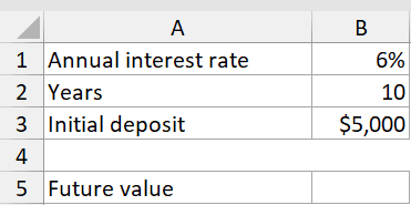
I want to find out what a one-time $5,000 deposit will grow to at 6% over 10 years with no additional contributions.
Here is the formula:
=FV(B1,B2,,-B3)
The result is $8,954.24. Here is what each argument does.
- B1 is the annual rate (6%). Since the deposit just sits there for whole years, no rate adjustment is needed here.
- B2 is the number of years (10), which is the number of periods.
- The double comma skips the pmt argument completely. There are no regular payments in this example.
- -B3 enters the deposit as a negative number because it is money going out.
Pro Tip: In FV, money you pay in (pmt and pv) is entered as a negative number. This is how Excel distinguishes cash outflows from returns. If you enter a positive pmt, FV returns a negative, confusing result.
Example 2: Future Value of Monthly Savings
Here’s another practical scenario.
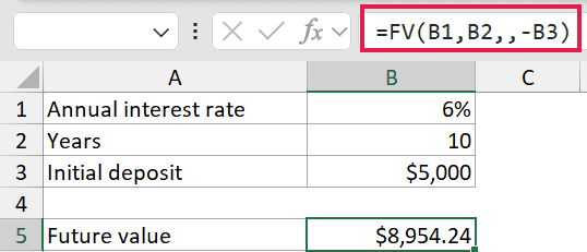
Below is the dataset. Labels in column A, values in column B. The inputs are an annual interest rate, a number of years, and a monthly contribution amount.
I want to see what $300 per month saved at 6% for 5 years will add up to.
Here is the formula:
=FV(B1/12,B2*12,-B3)
The result is $20,931.01. The key here is matching the rate and the period count to the payment frequency.
- B1/12 converts the annual rate into a monthly rate.
- **B2*12** turns years into months so the period unit matches.
- -B3 is the monthly contribution entered as a negative (money going out).
When the payments are monthly, both rate and nper have to be on a monthly basis. That is the most common FV mistake, so always double-check those two arguments. If you want to figure out how many periods it takes to reach a goal instead, that is what the NPER function is for.
Example 3: Beginning vs End of Period
Let’s see how much timing actually matters.
Below is the dataset. Labels in column A, values in column B. The inputs are an annual rate, years, and a monthly contribution. Row 5 will show the end-of-period result, and row 6 will show the beginning-of-period result.
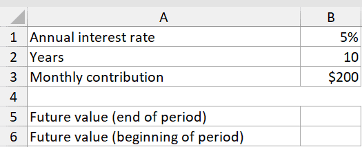
I want to compare what happens when you deposit at the end of each month versus the start.
Here are the formulas:
=FV(B1/12,B2*12,-B3,0,0)
=FV(B1/12,B2*12,-B3,0,1)
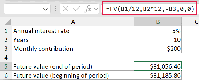
Paying at the end of each period gives $31,056.46, and paying at the start gives $31,185.86. The last argument is the type. 0 means the payment lands at the end of the period, 1 means the beginning.
When you pay at the start, each deposit earns one extra period of interest. The difference looks small month to month, but it adds up over time.
Pro Tip: The pv argument here is 0, meaning you are starting from nothing. Including it explicitly (rather than omitting it) is required when you need to reach the type argument, since both pv and type sit after pmt in the syntax.
Example 4: Lump Sum Plus Monthly Contributions
Let’s step it up with a more complex use case.
Below is the dataset. Labels in column A, values in column B. The inputs are an annual rate, years, a monthly contribution, and a current savings balance already on hand.
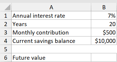
I want to find the future value when someone already has $10,000 saved and adds $500 per month at 7% for 20 years.
Here is the formula:
=FV(B1/12,B2*12,-B3,-B4)
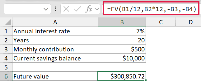
The result is $300,850.72. Both pmt and pv are negative because both are money going in.
- -B3 is the $500 monthly contribution (money out each month).
- -B4 is the $10,000 starting balance (money out up front).
FV compounds both and returns the total future value. The existing lump sum contributes a big chunk of that final number because it has 20 years to grow. If you want to calculate the fixed payment needed to reach a savings goal instead, the PMT function works the other way around.
Example 5: Compare Contribution Amounts at Once
Now here is where Excel 365 makes this really convenient.
Below is the dataset. Column A holds a list of monthly contribution amounts from $100 to $700, and column B will show the future value for each.
I want to see the 5-year future value at 6% for every contribution amount in the list, all from a single formula.
Here is the formula:
=FV(0.06/12,60,-A2:A8)
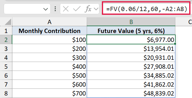
The formula spills a result for each of the seven rows. The $100 row comes out to about $6,977. The $700 row is about $48,840.
By feeding the range A2:A8 into the pmt argument, one formula handles all seven scenarios at once. The rate (6% annual, so 0.06/12) and the term (60 months) stay fixed. This is a clean way to build a quick comparison table without copying a formula down. For contributions that grow over time rather than staying fixed, check out growing annuity calculations in Excel.
Tips & Common Mistakes
- Match rate and nper to the same period. Monthly contributions need rate/12 and years*12. Forgetting this is the most common FV error and will give a wildly wrong answer.
- pmt and pv are negative. Money you put in is cash going out, so both arguments take negative values. FV then returns a positive future value. A positive pmt gives you a negative result, which is confusing.
- Use type 1 for beginning-of-period payments. If you are modeling something like a rent-style savings plan where you deposit at the start of each month, the type argument bumps the result up slightly.
- Use FVSCHEDULE for variable rates. FV assumes a constant rate throughout. If the interest rate changes from period to period, the FVSCHEDULE function handles that instead.
- The double-comma trick. If you have a lump sum but no regular payment, use a double comma to skip pmt and jump straight to pv:
=FV(rate,nper,,-pv). Leaving it blank is fine; just don’t put a zero there unless you want to be explicit.
The FV function is straightforward once you get the sign convention down. Enter what goes in as negative, match your rate and periods to the same time unit, and the function does the rest. Whether you are projecting a single lump sum, a stream of contributions, or both together, FV gives you the answer in one formula.
Related Excel Functions / Articles: