If you want to write your own custom function in Excel without touching VBA, the LAMBDA function is what you’re looking for. It lets you wrap a calculation into a reusable formula using plain parameter names.
LAMBDA is a Microsoft 365 only function, so it won’t work in Excel 2021 or earlier. On its own it returns whatever its calculation returns. Pair it with MAP, BYROW, or REDUCE to run it across a range, and the results spill into the cells below.
In this article, I’ll show you how to use LAMBDA on its own and alongside the helper functions that run it across a range.
LAMBDA Function Syntax in Excel
The LAMBDA function takes one or more parameter names, then a calculation that uses those parameters.
=LAMBDA([parameter1, parameter2, ...], calculation)
- parameter1, parameter2, … (optional) – the input names you make up, like
l,w, oracc. You can have up to 253 of them. - calculation (required) – the formula that runs, using the parameter names you defined.
A bare LAMBDA sitting in a cell returns a #CALC! error. To make it calculate, you add the input values in parentheses right after it, like =LAMBDA(x,x+1)(5).
When to Use LAMBDA Function
Here are some common situations where LAMBDA is the right tool:
- When you want to build your own reusable function without writing VBA.
- When a calculation is long and you want to name it once in the Name Manager and call it everywhere.
- When you need to run a custom calculation across an entire column with MAP.
- When you want to sum or process each row of a table with BYROW.
- When you need a running total or a single rolled-up value using SCAN or REDUCE.
Example 1: Call a LAMBDA Directly to Calculate Area
Let’s start with a simple example that shows how a LAMBDA gets called on its own.
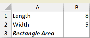
Below is a small parameter card. Cell B1 holds the length, B2 holds the width, and B3 is where we want the rectangle area.
We want to multiply length by width using a LAMBDA we define right in the cell.
Here is the formula:
=LAMBDA(l,w,l*w)(8,5)
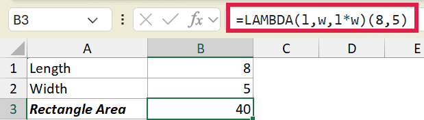
The first part, LAMBDA(l,w,l*w), defines a function with two inputs named l and w. The (8,5) right after it passes 8 and 5 into those inputs.
So the formula returns 8 times 5, which is 40. Without that (8,5) call at the end, the cell would just show a #CALC! error.
Pro Tip: If you plan to reuse this calculation, define it in the Name Manager as a named formula like RECTAREA. Then you can simply type =RECTAREA(8,5) anywhere in the workbook.
Example 2: Build a Full Name With a Text LAMBDA
A LAMBDA doesn’t have to do math. Here’s one that joins text.
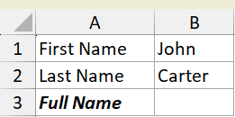
Below is another parameter card. B1 has the first name, B2 has the last name, and B3 is where we want the full name.
We want to join the first and last name with a space in between.
Here is the formula:
=LAMBDA(f,s,f&" "&s)("John","Carter")
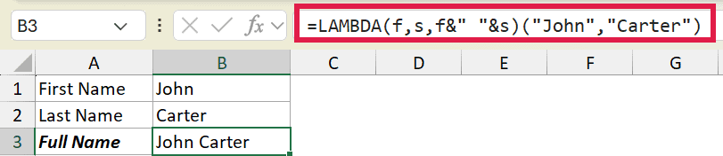
The LAMBDA defines two inputs, f and s. Inside, it joins them with &" "& so there’s a space between the two names.
The ("John","Carter") at the end passes the two text values in, and the formula returns “John Carter”.
Pro Tip: Parameter names can’t contain spaces or periods. Stick to simple names like f, s, first, or last and you’ll be fine.
Example 3: Apply a Discount to a Whole Column With MAP
Now let’s run a LAMBDA across a range using MAP. This is where it gets useful.
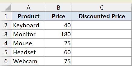
Below is a small product list. Column A has the product, column B has the price, and column C is where we want the discounted price.
We want to knock 10% off every price in one go.
Here is the formula:
=MAP(B2:B6,LAMBDA(p,p*0.9))
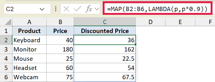
MAP walks through each value in B2:B6 and hands it to the LAMBDA as p. The LAMBDA then returns p*0.9, which is the price with 10% off.
The results spill down from C2 automatically. This is a dynamic array formula, so you write it once and every row fills in on its own.
Example 4: Sum Each Row With BYROW
Here’s another helper function. BYROW runs a LAMBDA once per row instead of once per value.
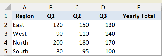
Below is a quarterly sales table. Each region has Q1, Q2, and Q3 figures, and column E is where we want the yearly total.
We want to add up the three quarters for each region in a single formula.
Here is the formula:
=BYROW(B2:D5,LAMBDA(row,SUM(row)))
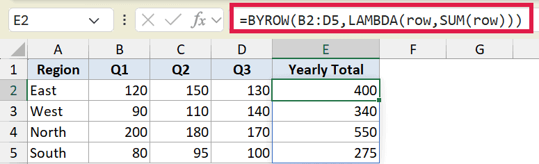
BYROW passes each row of B2:D5 into the LAMBDA as row. The LAMBDA then runs SUM(row) to add the three quarter values together.
The yearly totals spill down column E, one per region. No need to copy a SUM formula down four times.
Example 5: Running Total With SCAN
SCAN is great when you want a running total that grows as it goes down the list.
Below is a monthly sales table. Column A has the month, column B has the sales, and column C is where we want the running total.
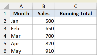
We want each row to show the total of all sales up to and including that month.
Here is the formula:
=SCAN(0,B2:B6,LAMBDA(acc,v,acc+v))
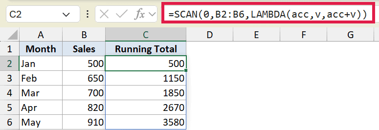
SCAN starts at 0 (the first argument). It then walks down B2:B6, and for each value it runs the LAMBDA with two inputs: acc (the total so far) and v (the current value).
Each step returns acc+v, so the total carries forward. The running totals spill down column C from January through May.
Pro Tip: When a LAMBDA takes an accumulator, the common naming convention is acc for the running result and v for the current value. It keeps SCAN and REDUCE formulas easy to read.
Example 6: Collapse an Array to One Value With REDUCE
Where SCAN shows every step, REDUCE gives you just the final number. It’s perfect for rolling a range up into one value.
Below is a horizontal list of cart item prices in B1:E1. Cell A2 is labeled “Total Cart Value” and B2 is where we want the answer.
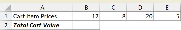
We want to add up all four prices into a single total.
Here is the formula:
=REDUCE(0,B1:E1,LAMBDA(acc,v,acc+v))
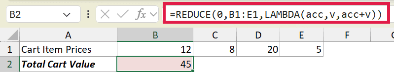
REDUCE works like SCAN but only returns the last result. It starts at 0, walks across B1:E1, and adds each value to the accumulator acc.
When it reaches the end, it returns the single total. Here that’s 12 + 8 + 20 + 5, which comes to 45 in cell B2.
Tips & Common Mistakes
- LAMBDA is Microsoft 365 only. It does not exist in Excel 2021, 2019, or earlier, and there’s no legacy fallback. If you share the file with someone on an older version, the formula won’t work for them.
- A bare LAMBDA returns #CALC!. If you type
=LAMBDA(x,x+1)and press Enter, you’ll get an error. You have to call it by adding the inputs in parentheses, like=LAMBDA(x,x+1)(5). - Parameter names can’t have spaces or periods. Use names like
acc,v,first, orrate. A name likefirst nameormy.valuewill throw an error. - For reuse, name it in the Name Manager. Defining the LAMBDA in-cell is fine for one-offs, but for a calculation you’ll use a lot, save it as a named formula so you can call it like any built-in function.
- Use the right helper for the job. MAP processes each value, BYROW and BYCOL work on whole rows or columns, SCAN gives a running result, and REDUCE collapses everything to one value.
That covers how LAMBDA works, both on its own and with the helper functions that run it across a range. Start with the direct in-cell calls to get comfortable with parameters, then move on to MAP, BYROW, SCAN, and REDUCE for real data.
Once you’re comfortable, defining your LAMBDA in the Name Manager turns it into your own custom function you can reuse anywhere in the workbook.
Related Excel Functions / Articles: