
If you want to do something when a cell contains a certain word, you cannot just use =IF(C2="urgent","Rush","Standard"). And this is because that test asks whether the cell IS urgent, not whether the word appears somewhere inside it.
An exact test like that belongs with comparing two cells. But nothing to worry about. Checking for text inside a cell is easy once you pick the right approach, and in this article I’ll show you six ways to do it.
Method #1: Use the ISNUMBER and SEARCH Functions to Check If a Cell Contains Specific Text in Excel
This is the combination I’d reach for by default, and the one most people are actually looking for. It ignores case, and it’s the only method here that handles the whole column with a single formula.
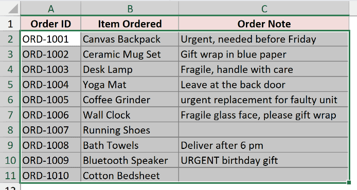
Below I have a list of orders. Column C holds the note the customer left, and I want to know which notes mention the word “urgent” anywhere inside them.
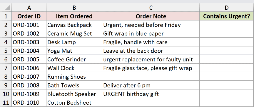
Here is the formula:
=ISNUMBER(SEARCH("urgent",C2:C11))
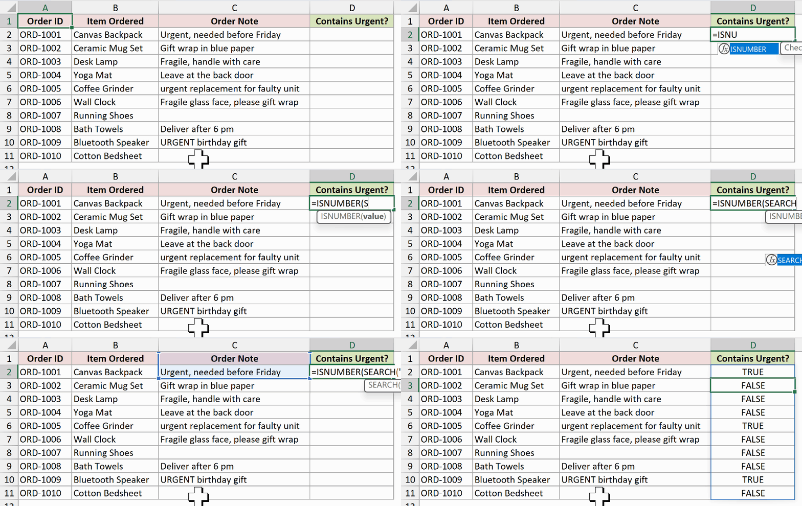
You get TRUE for ORD-1001, ORD-1005, and ORD-1009. Every other row gives you FALSE, including the two rows where the note is blank.
How does this formula work?
The SEARCH function looks for “urgent” inside each note. When it finds the word, it returns the position it starts at, so a hit is always a number.
When it doesn’t find the word, SEARCH returns a #VALUE! error instead. So the whole test comes down to one thing: did SEARCH hand back a number or not?
That’s what ISNUMBER answers. It turns any number into TRUE and anything else, error included, into FALSE.
Notice that I fed the formula the whole range C2:C11 instead of a single cell. In Excel 365 the formula spills down the column on its own, so you write it once in D2 and you’re done.
Note: SEARCH matches text anywhere inside the cell, including inside longer words. Searching for “gift” would also match “gifted” and “gifts”. If you only want the standalone word, search for ” gift ” with spaces around it.
TRUE and FALSE are fine, but you’ll usually want your own labels. Wrap the whole thing in IF and say what each outcome should return:
=IF(ISNUMBER(SEARCH("urgent",C2:C11)),"Rush","Standard")
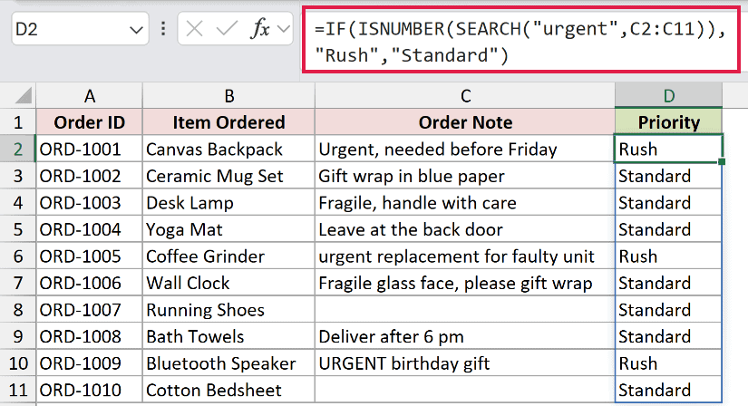
Now you get “Rush” on the same three orders and “Standard” on the other seven. IF handles ranges too, so this version spills down the column just like the first one.
Method #2: Use the COUNTIF Function With Wildcards to Check If a Cell Contains Specific Text in Excel
Here’s another way to do this. If you already think in COUNTIF, this one reads more naturally than nesting two functions.
Same dataset. Column C has the order notes, and I want to mark the ones that mention “urgent”.
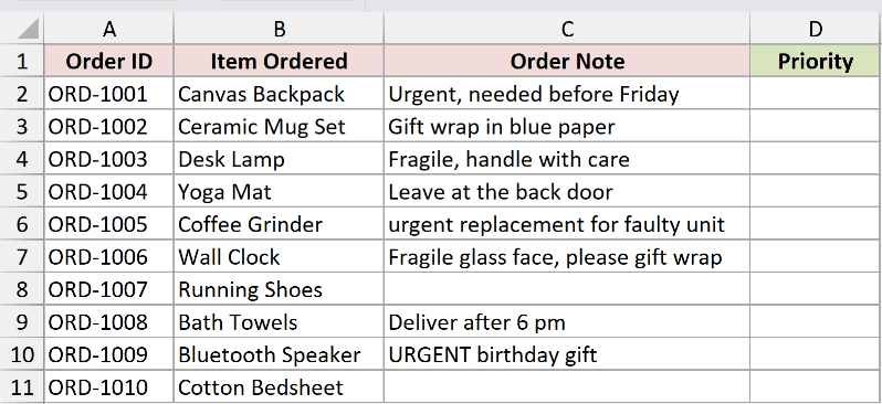
Here is the formula:
=IF(COUNTIF(C2,"*urgent*")>0,"Rush","Standard")
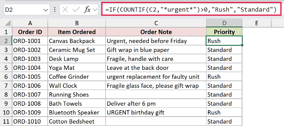
You get “Rush” on ORD-1001, ORD-1005, and ORD-1009. That’s the same answer Method #1 gave you.
How does this formula work?
The asterisks are wildcards. An asterisk stands for any number of characters, so "*urgent*" reads as “anything, then urgent, then anything”.
The COUNTIF function checks cell C2 against that pattern and returns 1 if it matches and 0 if it doesn’t. Testing for >0 turns that count into a TRUE or FALSE, and IF gives it a label.
There is one real difference from Method #1. COUNTIF’s first argument wants a reference, not an array, so this formula won’t spill.
Writing =COUNTIF(C2:C11,"*urgent*") gives you the single number 3, not ten separate answers. So enter this one in D2 and fill it down the column.
Note: COUNTIF wildcards only match text values. If your column holds actual numbers, "*5*" will not find 15. Convert the numbers to text first, or use the SEARCH approach from Method #1 instead.
Method #3: Apply the FIND Function to Check If a Cell Contains Text With Matching Case in Excel
The first two methods don’t care about capitalization. Sometimes that matters, and this is where FIND comes in.
Same order notes. But look closely at column C: the word urgent is written three different ways. ORD-1001 has “Urgent”, ORD-1005 has “urgent”, and ORD-1009 has “URGENT”.
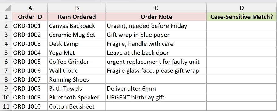
Say I only want the notes where it’s capitalized exactly as “Urgent”. Here is the formula:
=ISNUMBER(FIND("Urgent",C2:C11))
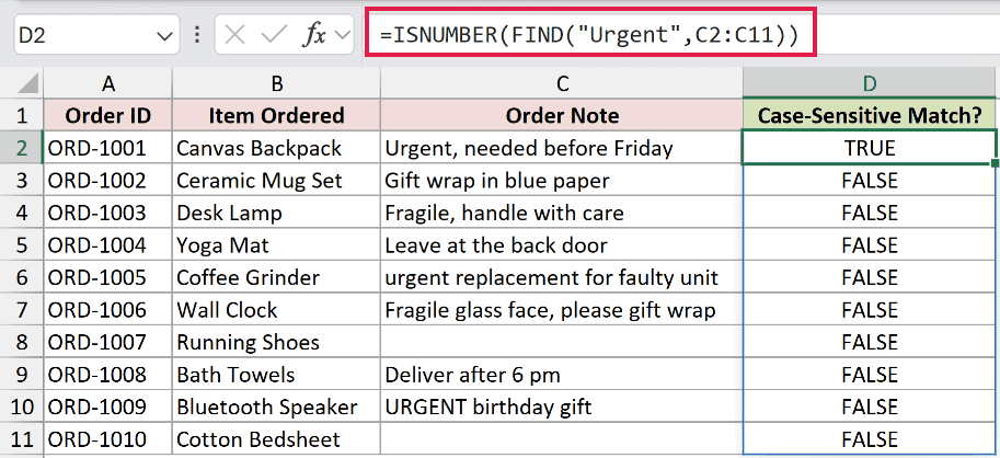
Only ORD-1001 comes back TRUE. The other nine rows are FALSE, including the two that clearly mention urgent in a different case.
How does this formula work?
FIND works exactly like SEARCH. It returns the starting position of the text it finds, and a #VALUE! error when it finds nothing. ISNUMBER turns that into TRUE or FALSE.
The one difference is that the FIND function is case-sensitive. To FIND, “Urgent” and “urgent” are two different pieces of text, which is why the count drops from three hits to one.
Like SEARCH, FIND spills in Excel 365, so this stays a single formula for the whole column.
Note: There’s a second difference worth knowing. SEARCH accepts the * and ? wildcards, and FIND does not. So FIND is stricter in both senses: it matches case, and it treats an asterisk as a literal asterisk. There’s more on this in our guide to the difference between SEARCH and FIND.
There is no case-sensitive version of COUNTIF, so if case matters, Method #2 is off the table.
Method #4: Use the ISTEXT Function to Check If a Cell Contains Any Text in Excel
Everything so far looks for one specific word. Sometimes the question is simpler: does this cell have any text in it at all?
Same dataset, different goal. Two of my orders came in with no note at all, and I want to spot them.
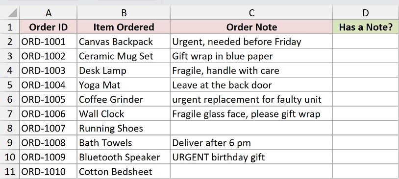
Here is the formula:
=ISTEXT(C2:C11)
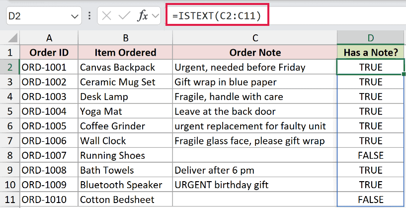
Eight rows return TRUE. ORD-1007 and ORD-1010 return FALSE, which are exactly the two orders that came in without a note.
How does this formula work?
The ISTEXT function asks one question: is this value text? You don’t give it a search term, and there are no wildcards or capitalization to think about.
It returns FALSE for empty cells, and also for numbers and dates, since Excel stores those as numbers rather than text. Like the other IS functions, it spills across a range in Excel 365.
Note: There’s one trap here. If a cell holds a formula that returns an empty string, such as =IF(A2=””,””,A2), the cell looks blank but ISTEXT returns TRUE. An empty string is still text as far as Excel is concerned. Use ISBLANK if you need truly empty cells.
Method #5: Combine SUMPRODUCT and SEARCH to Check If a Cell Contains Text From a List in Excel
If you’d rather not rewrite your formula every time the keyword changes, this one is for you. It checks each note against a whole list of words at once.
Here’s the same order data, and this time I’ve put three keywords in F2:F4: urgent, fragile, and gift wrap. I want to flag any note that mentions any one of them.
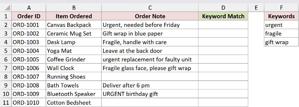
Here is the formula:
=IF(SUMPRODUCT(--ISNUMBER(SEARCH($F$2:$F$4,C2)))>0,"Flag","No")
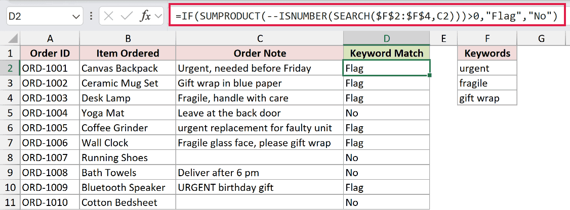
Six orders get flagged: ORD-1001, ORD-1002, ORD-1003, ORD-1005, ORD-1006, and ORD-1009. The remaining four come back “No”.
How does this formula work?
Because I handed SEARCH a range of three keywords, it checks the note against all three at once and returns three results rather than one.
ISNUMBER turns those three results into TRUE or FALSE. The double minus in front, called a double unary, converts them into 1s and 0s, because SUMPRODUCT ignores TRUE and FALSE but happily adds numbers.
SUMPRODUCT then adds those three 1s and 0s into a single count of how many keywords the note matched.
That count is why the test is >0 rather than =1. Look at ORD-1006: its note mentions both “Fragile” and “gift wrap”, so its count is 2, and =1 would have skipped it.
SUMPRODUCT collapses everything down to one number per row, so this formula doesn’t spill. Enter it in D2 and fill it down.
Note: On Excel 365 you can get a spilling version with BYROW: =BYROW(C2:C11,LAMBDA(n,OR(ISNUMBER(SEARCH($F$2:$F$4,n))))). You write it once in D2 and you don’t have to fill anything down. If you want to check for an exact match against a list rather than a word inside a sentence, see how to check if a value is in a list.
Method #6: Apply Conditional Formatting to Highlight Cells That Contain Text in Excel
If you’d rather see the answer than read it, skip the helper column entirely and let Conditional Formatting color the rows for you.
Same order data. I want to highlight the entire row of any order whose note mentions “fragile”.
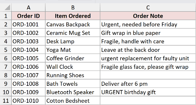
Here are the steps to highlight the rows that contain text:
- Select the range A2:C11, starting from cell A2.
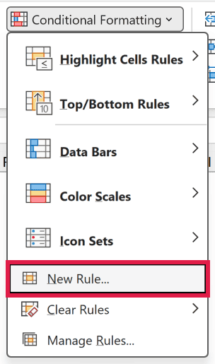
- On the Home tab, click Conditional Formatting, then click New Rule.
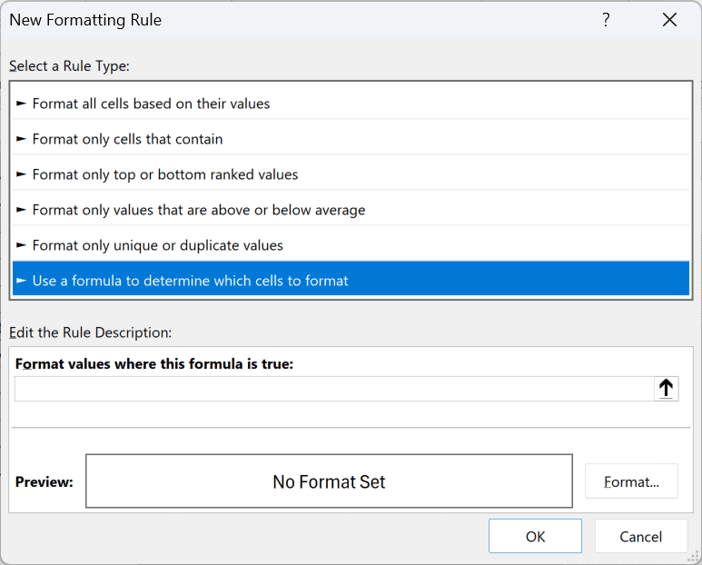
- In the New Formatting Rule dialog box, select “Use a formula to determine which cells to format”.
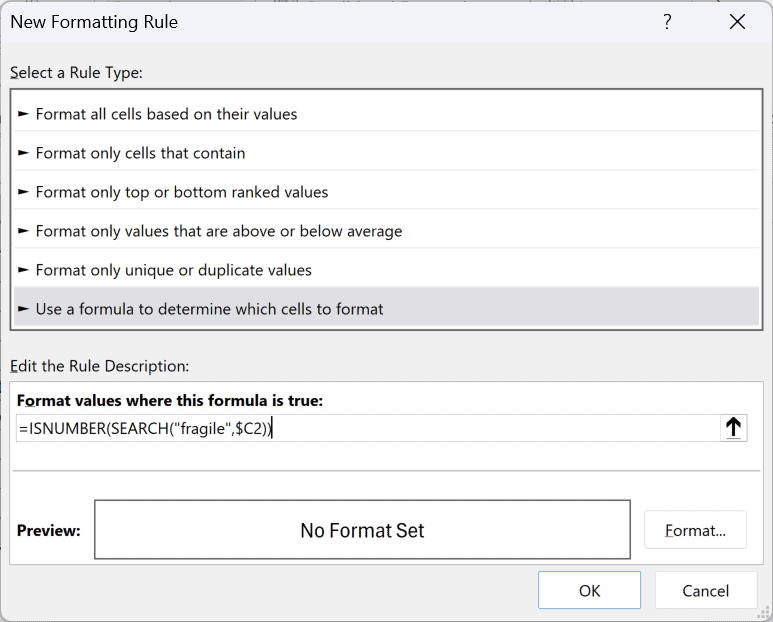
- In the formula box, enter =ISNUMBER(SEARCH(“fragile”,$C2))
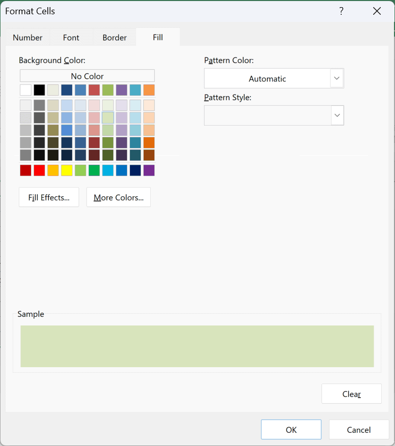
- Click the Format button, go to the Fill tab, pick a color, and click OK.
- Click OK to apply the rule.
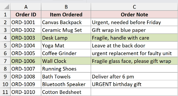
The rows for ORD-1003 and ORD-1006 light up, and nothing else does. Those are the two notes that mention fragile.
The formula is the same test from Method #1, with one change that does all the work.
The reference $C2 locks the column but leaves the row free. So every row checks its own note in column C, while the highlight covers columns A through C.
Note: Write the formula against the first row of your selection. Excel reads $C2 relative to the top-left cell of the Applies to range, so if your rule covers $A$2:$C$11 but the formula points at $C5, the highlighting lands on the wrong rows.
Additional Notes About Checking If a Cell Contains Text in Excel
- Blank cells give you FALSE, not an error. SEARCH on an empty cell does return a
#VALUE!error, but ISNUMBER swallows it and hands back FALSE. So you don’t need IFERROR around any of these formulas. - To search for a literal
*or?, put a tilde in front of it.SEARCH("~*",C2)finds an actual asterisk. The same goes for COUNTIF criteria. Without the tilde, Excel reads them as wildcards. - Put your keyword in a cell instead of hardcoding it. Swap
"urgent"for$G$1and you can change what you’re looking for without editing a single formula. Lock the reference with dollar signs if you’re filling down. - Everything here is case-insensitive except FIND. SEARCH, COUNTIF, and even a plain
=comparison all ignore capitalization. If case matters, FIND is your only option out of this set.
Frequently Asked Questions
Does SEARCH work with wildcards when checking if a cell contains text?
Yes. SEARCH accepts both * (any number of characters) and ? (a single character). So SEARCH("gift?wrap",C2) matches “gift wrap” and “gift-wrap”. FIND does not accept wildcards at all.
How do I count or sum the rows where a cell contains certain text?
That’s a different job from flagging each row. For counting, use COUNTIF with wildcards across the whole range, like =COUNTIF(C2:C11,"*urgent*"). We cover it properly in our guide to COUNTIF with a partial match. For adding up a column, SUMIF takes the same wildcard criteria.
Why does my formula return FALSE when the cell is empty instead of an error?
Because ISNUMBER catches the error before you see it. SEARCH does throw #VALUE! on a blank cell, but ISNUMBER only asks “is this a number?” An error isn’t a number, so you get FALSE.
How do I check if a cell contains a number instead of text?
Use ISNUMBER on the cell directly: =ISNUMBER(C2). That’s a different question from Method #1, where ISNUMBER was checking SEARCH’s output rather than the cell itself.
Can I check if a cell contains text and return the keyword that matched?
Yes, with a small change to Method #5. Replace the SUMPRODUCT wrapper with INDEX and MATCH: =IFERROR(INDEX($F$2:$F$4,MATCH(TRUE,ISNUMBER(SEARCH($F$2:$F$4,C2)),0)),""). It returns the first keyword that matched, or a blank when nothing did.
This one handles an array internally, so on Excel 365 you just press Enter. On older versions, confirm it with Ctrl + Shift + Enter.
Conclusion
So those are six ways to check if a cell contains text in Excel. Five of them give you an answer in a helper column, and the last one skips the column and colors the rows instead.
If you’re not sure which one to pick, start with ISNUMBER(SEARCH()). It ignores case, it handles blanks without complaining, and one formula covers your whole column.
Reach for FIND when capitalization matters, ISTEXT when you just want to know whether a cell has anything in it, and Conditional Formatting when you’d rather see the answer than read it.
Other Excel articles you may also like:
