
If you have taken out a car loan and want to see exactly where each monthly payment goes, an amortization schedule is what you need. It splits every payment into the part that covers interest and the part that reduces what you still owe.
Building one from scratch sounds like heavy math, but Excel handles the hard part with a couple of built-in functions. You set up the formulas once, then fill them down through the loan term.
In this tutorial, I’ll walk you through building a full car loan amortization schedule step by step.
If you just want a quick number without building anything, our loan amortization schedule calculator does it for you, but building it yourself shows you exactly how the math works.
📁 Click here to download the Car Loan Amortization Schedule Template
Step 1: Set Up the Car Loan Inputs
Every amortization schedule starts with the loan details. Keeping them in their own labeled cells means changes to the loan amount or rate update the existing schedule. If you change the term, you also need to adjust the number of payment rows.
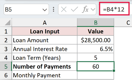
For this example, I’m using a car loan of $28,500 at 6.5% APR over a 5-year term. Here is how I’ve laid out the inputs.
- A2: Loan Amount, B2: 28500
- A3: Annual Interest Rate, B3: 6.5%
- A4: Loan Term (Years), B4: 5
- A5: Number of Payments, B5: =B4*12
- A6: Monthly Payment, B6: (we’ll add this in Step 2)
The formula in B5 multiplies the term in years by 12 to give the total number of monthly payments, which comes to 60.
Note: Enter the interest rate as an annual figure and let the formulas divide it by 12. If you type the monthly rate directly, it’s easy to forget later what the real APR was.
Step 2: Calculate the Monthly Payment with the PMT Function
Before you can split anything into interest and principal, you need the fixed monthly payment. Excel’s PMT function works this out from the rate, the number of payments, and the loan amount.
In cell B6, enter this formula:
=PMT(B3/12, B5, -B2)
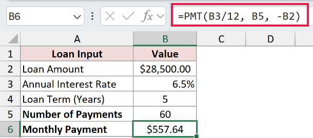
This returns $557.64, the amount you pay every month for all 60 months.
How does this formula work?
The first argument, B3/12, is the interest rate per period. Since B3 holds the annual rate, dividing by 12 gives the monthly rate.
The second argument, B5, is the total number of payments, which is 60. The third argument is the loan amount, entered as -B2 so the payment comes back as a positive number.
PMT treats money you receive as positive and money you pay out as negative, so flipping the sign on the loan keeps the result readable.
Step 3: Build the Amortization Schedule Structure
Now set up the table that will hold the payment-by-payment breakdown. Each row is one monthly payment, and each column tracks a piece of that payment.
Starting in row 8, add these six column headers.
- A8: Payment #
- B8: Beginning Balance
- C8: Payment
- D8: Interest
- E8: Principal
- F8: Ending Balance
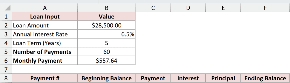
The idea is simple. Each month you start with a balance, make your fixed payment, some of it covers interest, the rest reduces the balance, and you end with a smaller balance that carries into the next row.
Step 4: Calculate Interest and Principal for Each Payment
This is the heart of the schedule. Let’s build the first payment row (row 9) one cell at a time, then reuse it for every month after.
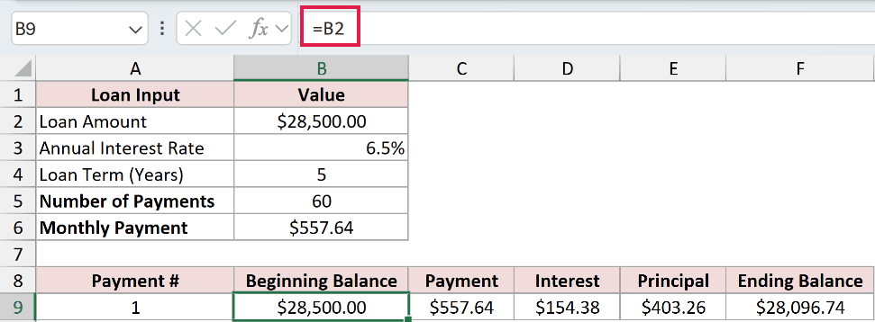
Start with the payment number and the beginning balance. In A9 enter 1, and in B9 pull in the original loan amount.
=B2
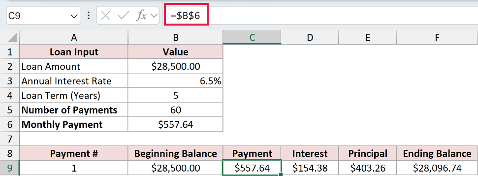
Next, bring in the fixed monthly payment. In C9, reference the payment cell with an absolute reference so it stays locked when you fill down.
=$B$6
Now the interest. The interest for the month is the beginning balance times the monthly rate. In D9, enter this.
=B9*$B$3/12
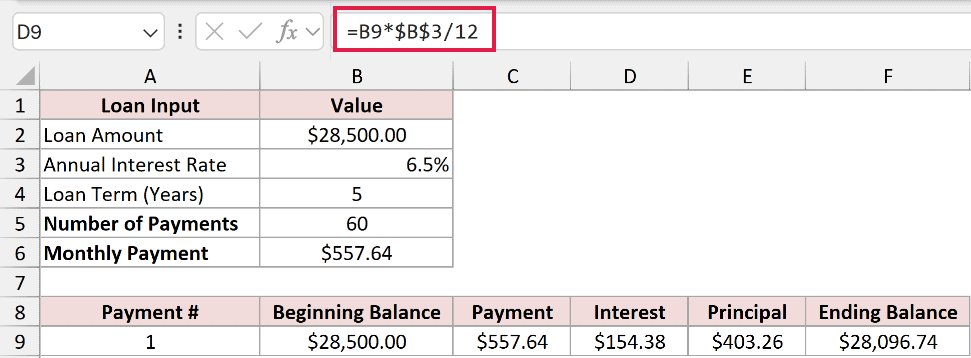
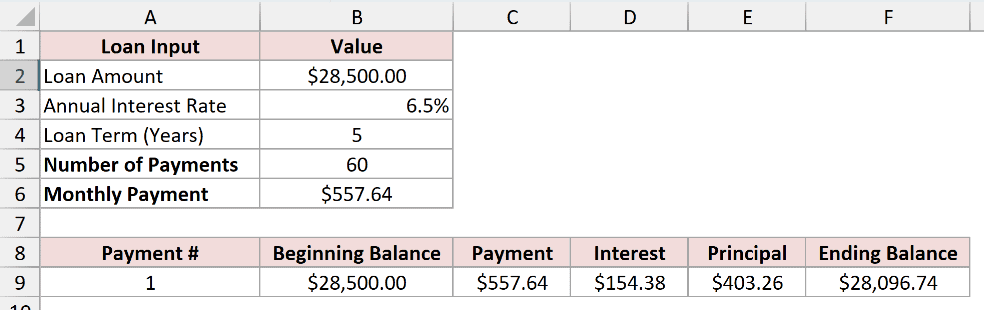
For the first payment this comes to $154.38. That is what the lender charges in interest before any of your payment touches the balance.
The principal is whatever is left of your payment after interest. In E9, subtract interest from the payment.
=C9-D9
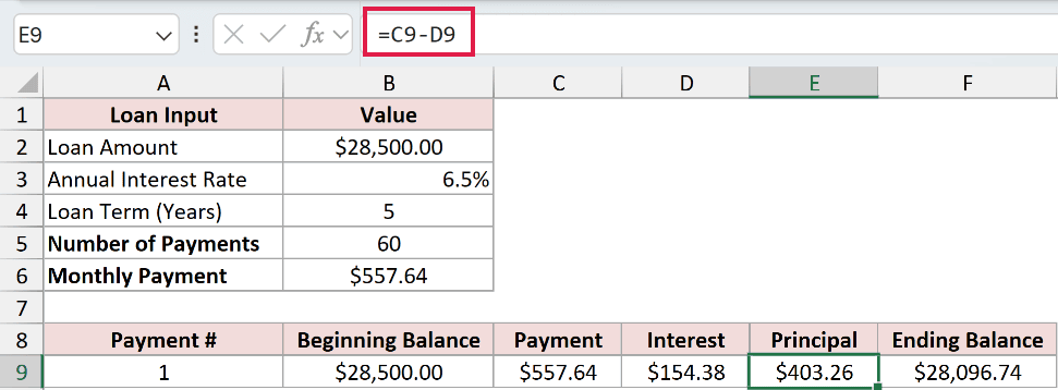
That leaves $403.26 going toward the actual balance in month one. Finally, the ending balance is the beginning balance minus the principal you just paid. In F9, enter this.
=B9-E9
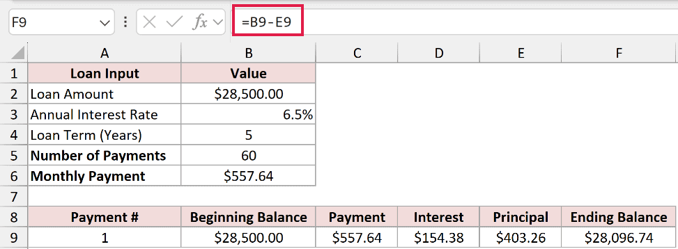
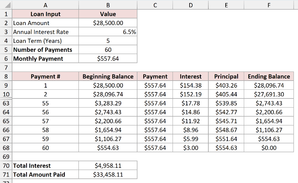
The first row now shows a beginning balance of $28,500, $154.38 in interest, $403.26 in principal, and an ending balance of $28,096.74.
Note: Excel also has IPMT and PPMT functions that return the interest and principal for any given payment directly. The beginning-balance method used here is easier to follow and self-checks, because the ending balance has to reach zero on the last row.
Step 5: Fill Down the Schedule for the Full Loan Term
The first row is a special case because its beginning balance comes straight from the loan amount. Every row after that starts with the previous row’s ending balance, so you build one more row and then fill the rest.
In row 10, set up the second payment so its formulas point at the row above.
- In A10, enter =A9+1 to count the payment number up by one.
- In B10, enter =F9 so the beginning balance equals the previous ending balance.
- In C10, D10, E10, and F10, copy the same formulas you used in row 9 (payment, interest, principal, and ending balance).
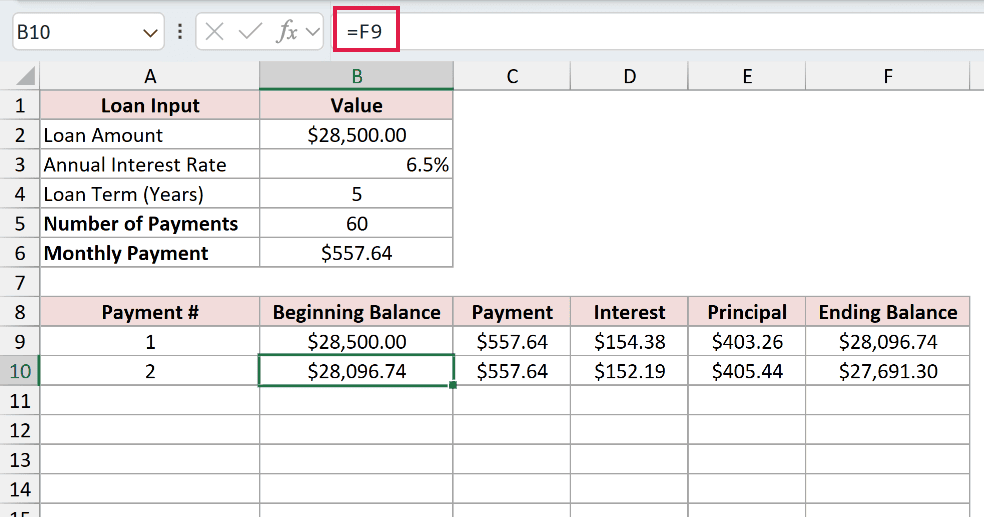
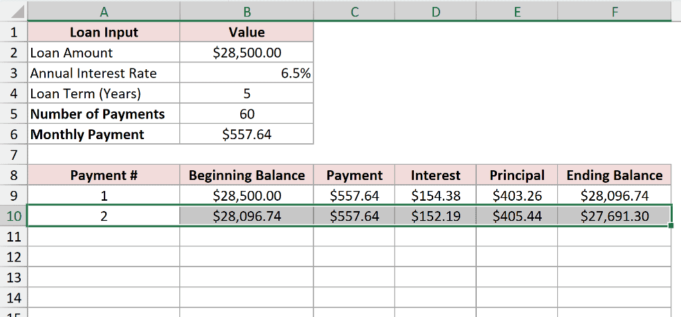
With row 10 done, select the range A10:F10, then drag the fill handle down (or copy and paste) to row 68. That gives you all 60 payments.
The real test that everything is correct is the ending balance on the last row. Payment 60 should leave a balance of $0.00.
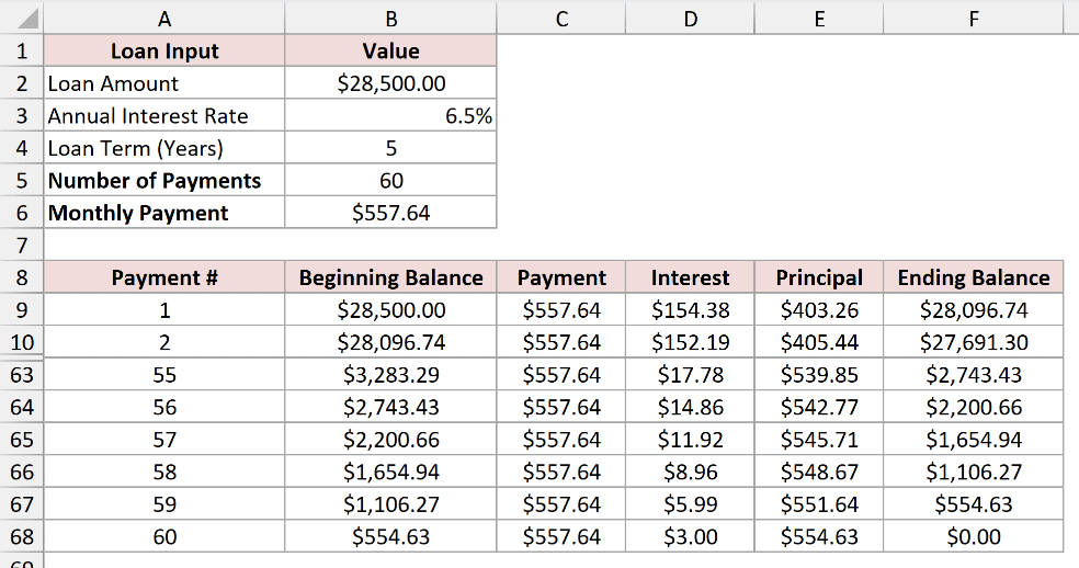
Note: Because of floating-point precision, the last row may show a tiny residual in scientific notation instead of an exact zero. That is normal. Format the Ending Balance column as Currency and it displays as $0.00. Don’t round every row’s ending balance, because repeated rounding can leave a few cents at the end.
Step 6: Add a Total Interest Summary
The schedule already tells the full story, but the number most people care about is how much the loan costs in interest overall. Add a quick summary below the table.
In a cell under the schedule, sum the entire interest column.
=SUM(D9:D68)
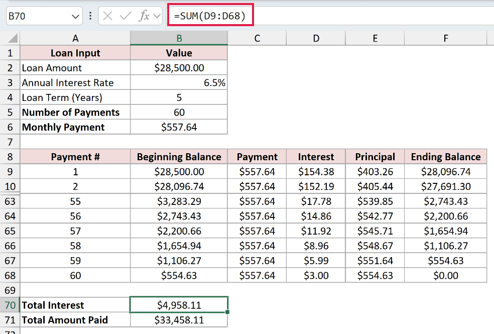
For this loan that comes to $4,958.11 in total interest. You can add the total amount paid the same way by summing the payment column, or just multiply the monthly payment by the number of payments.
=B6*B5
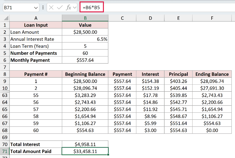
That returns $33,458.11, which is the $28,500 you borrowed plus the $4,958.11 in interest. Here is the finished schedule with the summary in place.
📁 Click here to download the Car Loan Amortization Schedule Template
Additional Notes About Building a Car Loan Amortization Schedule in Excel
- Because every formula points back to the input cells, changing the loan amount or rate updates the existing schedule instantly. If you change the term, refill the schedule to the new last payment and update the summary ranges.
- Format the money columns as Currency and the rate cell as a percentage so the numbers read clearly. Formatting does not change the math, only how it looks.
- The schedule assumes a fixed rate and equal monthly payments. If your loan has a promotional rate that changes later, you’d need a separate section for the second rate.
- Keep the number of payments and the term in sync. If you switch to a 6-year loan, update the term cell and refill the schedule down to row 80 to cover all 72 payments.
Frequently Asked Questions
How do I account for extra payments in a car loan amortization schedule?
Add an Extra Payment column, then change the ending-balance formula to also subtract that extra amount. Cap the ending balance at zero and stop later rows from calculating so the schedule doesn’t continue into negative balances.
What’s the difference between IPMT and PPMT in an amortization schedule?
IPMT returns the interest portion of a specific payment, while PPMT returns the principal portion of that same payment. Add the two together for any period and you get the full monthly payment.
Can I build a car loan amortization schedule without using the PMT function?
Yes, but you’d have to calculate the payment yourself with the annuity formula, which is more error-prone. PMT does the same math in one step, so there’s little reason to skip it.
Conclusion
Building a car loan amortization schedule in Excel comes down to one payment formula and a table that carries the balance forward each month.
Set up the inputs, get the payment with PMT, split each payment into interest and principal, then fill down until the balance hits zero.
Once it’s built, it’s reusable. Changes to the loan amount or rate recalculate the existing schedule and total interest. If you change the term, adjust the filled rows and summary ranges too.
Other Excel articles you may also like:
