
If you want to build a balance sheet in Excel, the whole thing rests on one simple rule: your assets have to equal your liabilities plus equity.
When those two sides don’t match, a figure may be entered or classified incorrectly, and that’s easy to miss in a long column of numbers. The good news is you can let Excel watch that rule for you.
In this tutorial I’ll set up a small retail balance sheet step by step, then add a check formula that tells you instantly whether it balances or how far off you are.
Step 1: Set Up the Assets Section
Everything starts with what the business owns. I’m using Sunrise Cycles, a small retail bike shop, so its assets are the cash in the bank, money customers still owe, stock on the shelves, and the shop equipment.
Put your labels in column A and the amounts in column B. Rows 1 and 2 hold a small header: the company name and statement title in row 1, and the “As of” date in row 2. Leave row 3 empty, then type the section title in A4 and list each asset below it. Here’s how I laid out the current assets first.
- In cell A4, type Assets as the section header.
- In A5:A7, type Cash, Accounts Receivable, and Inventory (at cost).
- In B5:B7, enter 12000, 6500, and 18500.
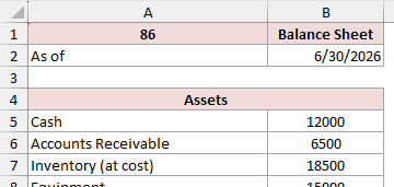
Notice the inventory is valued at product cost, not at what you’d sell it for. Use the inventory’s accounting cost from your records rather than its retail price. Depending on the applicable accounting rules, inventory may also need to be written down below cost.
Next come the fixed assets. The shop owns equipment worth 15,000, but gear loses value over time, so you subtract the depreciation built up so far.
- In A8 and A9, type Equipment and Less: Accumulated Depreciation.
- In B8, enter 15000. In B9, enter -3000 (a negative, since it reduces the total).
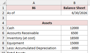
That depreciation number usually comes from a schedule. If you’re not sure how to work it out, the SLN function calculates straight-line depreciation for you, a common method for shop equipment.
Now total it up. In A10, type Total Assets, and in B10, add every asset with a single SUM.
=SUM(B5:B9)
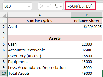
This returns 49000. The SUM covers B5 through B9, so the negative depreciation in B9 is subtracted automatically as part of the total.
Step 2: Set Up the Liabilities and Equity Sections
The other side of the sheet shows where the money came from. That splits into liabilities (what the business owes to others) and equity (what the owner has put in and earned). Leave a blank row after your assets, then build both sections below.
Start with liabilities. Sunrise Cycles owes its suppliers and still has a bank loan to pay off.
- In A12, type Liabilities as the section header.
- In A13 and A14, type Accounts Payable and Bank Loan.
- In B13 and B14, enter 9000 and 20000.
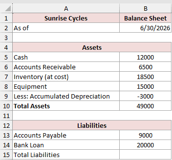
In A15, type Total Liabilities, and total the two amounts in B15.
=SUM(B13:B14)
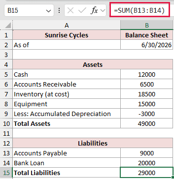
That gives you 29000. Now the equity section, right below the liabilities. This is the owner’s stake: the capital originally invested plus the profit kept in the business.
- In A17, type Equity as the section header.
- In A18 and A19, type Owner’s Capital and Retained Earnings.
- In B18 and B19, enter 15000 and 5000.
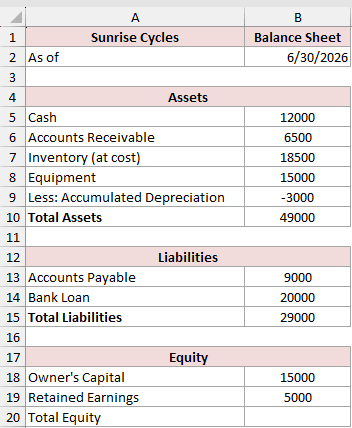
In A20, type Total Equity, and sum the two figures in B20.
=SUM(B18:B19)
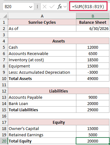
That returns 20000. Finally, combine the two sides into a single figure. In A22, type Total Liabilities & Equity, and in B22 add your two totals together.
=B15+B20
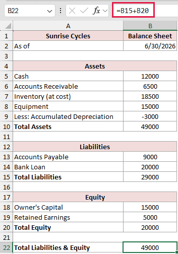
This gives you 49000, the same number as Total Assets. That match is the whole point of a balance sheet, and the next step makes Excel confirm it for you.
Step 3: Add the Balance Check Formula
Eyeballing two totals works until you have a long sheet and a typo hides in it. A small IF formula removes the guesswork. It compares Total Assets against Total Liabilities plus Equity, and reports back in plain words.
In A24, type Balance Check. In B24, enter the formula below.
=IF(B10=B15+B20,"Balanced","Off by "&TEXT(ABS(B10-(B15+B20)),"#,##0"))
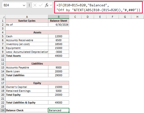
Because both sides equal 49000, the cell shows Balanced.
How does this formula work?
The IF checks whether B10 (Total Assets) equals B15 plus B20 (Total Liabilities plus Equity). If they match, it returns the text “Balanced”. If they don’t, it runs the second part instead.
That second part builds a message. ABS(B10-(B15+B20)) finds the gap between the two sides and drops any minus sign, so you always get a positive difference.
TEXT then wraps that number in the “#,##0” format so it reads with a thousands separator, and the “&” joins it onto the words “Off by “.
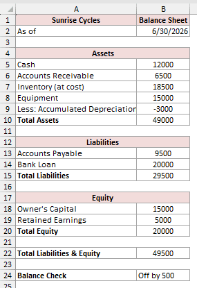
To see it in action, change B13 (Accounts Payable) from 9000 to 9500. Total Liabilities jumps, the two sides no longer agree, and the cell now reads Off by 500.
Note: If you name the total cells (select B10 and type Total_Assets in the Name Box, and so on), the formula reads =IF(Total_Assets=Total_Liabilities+Total_Equity,…). It behaves the same but is far easier to read months later.
Set B13 back to 9000 before you move on, so the sheet balances again.
Step 4: Format the Balance Sheet for Reporting
The numbers are right, but the sheet still looks like a rough draft. A few formatting touches turn it into something you’d be happy to hand to an accountant or a lender. None of this changes the values, only how they read.
Start with the numbers. Select the amount cells and apply the Accounting format so the figures line up by their decimal point and share a currency symbol.
- Select the amount cells in column B (B5:B22).
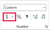
- On the Home tab, in the Number group, click the Accounting Number Format button (the dollar-sign icon).
Next, make the section headers and totals stand out so the eye can jump straight to them.
- Select the section headers (Assets, Liabilities, Equity) and the total rows, then press Ctrl + B on Windows or Command + B on Mac to bold them.
Add a top border above each total so it reads as a sum of the rows above it, the way printed statements do.
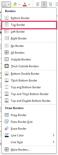
- Select the total cells, then on the Home tab click the arrow next to the Borders button and choose Top Border.
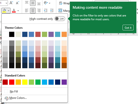
Finally, add a light fill behind the Total Assets and Total Liabilities & Equity rows. Those are the two numbers a reader checks first, so shading them makes the balance obvious at a glance.
- Select the two grand-total rows, then use the Fill Color button on the Home tab to apply a light shade.
Here’s the finished balance sheet with all four steps applied.
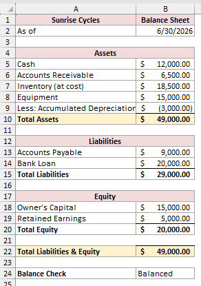
With that, the balance sheet is clean, readable, and still self-checking. Any future edit that throws it out of balance will show up in the Balance Check cell right away.
Additional Notes About the Balance Sheet Formula in Excel
- Keep every total as a SUM formula, never a typed-in number. If you paste a hard-coded total, the balance check can’t catch an error in the rows above it.
- Enter reductions like accumulated depreciation as negative values, not as a separate subtraction. That way a single SUM handles the whole column and nothing gets missed.
- Value inventory at cost, not selling price. Mixing the two is one of the most common reasons a first balance sheet refuses to balance.
- A balance sheet is a snapshot on one date. Put that date in a header cell so you don’t confuse this month’s version with last month’s.
- If your check shows a small “Off by” amount, look for rounding or a single mistyped figure first. Those account for most tiny mismatches.
- Once you have cents in the figures, compare rounded values instead of raw ones: =IF(ROUND(B10-(B15+B20),2)=0,”Balanced”,…). Excel stores decimals with a tiny amount of imprecision, so a sheet that is right to the penny can otherwise report “Off by 0”.
Frequently Asked Questions
What’s the basic balance sheet formula in Excel?
The core rule is Assets = Liabilities + Equity. In Excel you build each side with SUM formulas, then confirm they match. Nothing about it needs a special function beyond addition.
How do I make Excel flag it automatically if my balance sheet doesn’t balance?
Add an IF formula that compares the two totals, like =IF(B10=B15+B20,”Balanced”,”Off”). It updates the moment any figure changes, so you never have to re-check by hand.
Is there a free balance sheet template built into Excel?
Yes. Go to File, then New, and search for “balance sheet” in the template box. Building your own is still worth doing once, since you learn exactly where each number feeds into the totals.
Should I split assets and liabilities into current and non-current?
Most published balance sheets do. Add a Total Current Assets row after Inventory and a Total Current Liabilities row after your short-term debts, then have Total Assets add the two subtotals rather than the individual lines.
It also gives you the ratios a lender looks at, since the current ratio is current assets divided by current liabilities.
How do I make the Balance Check stand out when the sheet is off?
Select the Balance Check cell, go to Home, then Conditional Formatting, then New Rule, and choose to format cells that contain text starting with “Off”. Give it a red fill, and the cell turns red the moment the two sides stop matching.
Can I use SUBTOTAL instead of SUM for the section totals?
You can, and it helps if you plan to filter rows later. For a fixed statement like this, plain SUM is simpler and reads more clearly.
Conclusion
Building a balance sheet in Excel comes down to laying out assets on one side, liabilities and equity on the other, and totaling each with SUM.
The IF check formula is the piece that saves you, since it flags a mismatch the instant it happens instead of letting a typo slip through.
Start with the layout in Step 1, and by the time you reach the check formula you’ll have a sheet that keeps itself honest.
Other Excel articles you may also like:
