How to Divide in Excel

If you want to divide numbers in Excel, you’ll go looking for a DIVIDE function and there isn’t one. And this is because Excel handles division with a plain forward slash instead of a named function.

But nothing to worry about. Division is one of the easiest things to do in Excel once you know where the slash goes. In this article I’ll show you eight ways to divide, from a simple formula to Power Query.

Method #1: Using the Division Operator (/)

The forward slash is Excel’s division sign. You put it between two cell references, press Enter, and you have your answer.

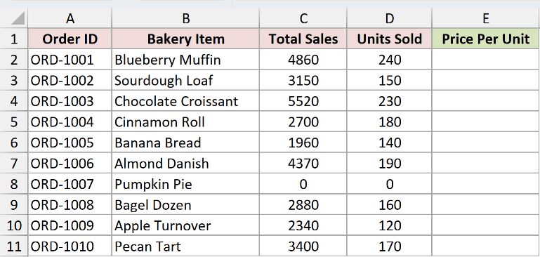
Below I have a bakery’s order data. Column C has the total sales for each item and column D has the number of units sold. I want the price per unit in column E.

Here is the formula for the first row:

=C2/D2

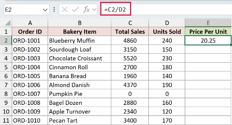
That gives 20.25, because 4860 divided by 240 is 20.25.

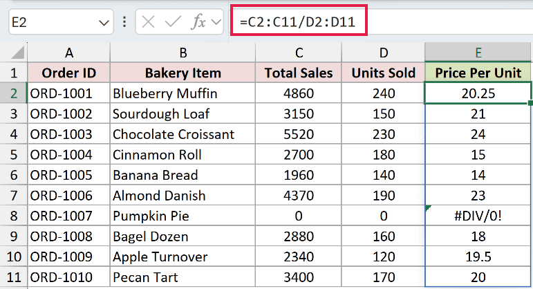
To do the whole column at once, point the same formula at both ranges instead of both cells:

=C2:C11/D2:D11

How does this formula work?

Excel divides the first cell of the left range by the first cell of the right range, then the second by the second, and so on down the pair.

You type it once in E2 and the results spill down the column on their own. There is nothing to drag and nothing to copy.

The prices come out as 20.25, 21, 24, 15, 14, 23, an error, 18, 19.5 and 20. That error on row 7 is the Pumpkin Pie, which hasn’t sold a single unit yet. Method #6 deals with it.

Note: The spilling range version needs Excel for Microsoft 365 or Excel 2021. On an older version, put =C2/D2 in E2 and double-click the little square at the bottom-right corner of the cell to copy it down.

Method #2: Using an Absolute Cell Reference ($)

Here’s another way to do this. Sometimes you’re not dividing column by column. You’re dividing every row by one single number that lives in one cell.

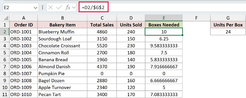
Below I have the same bakery data. The bakery packs everything in boxes of 24, and that 24 sits in cell G2. I want to know how many boxes each order fills.

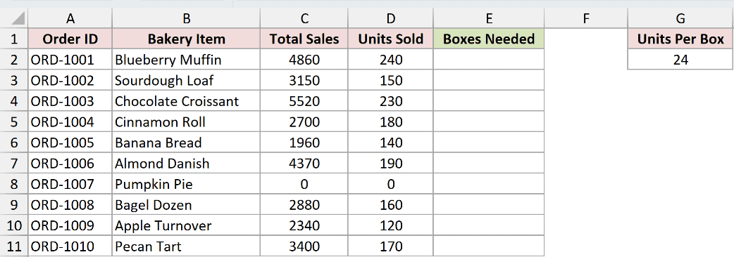
Here is the formula:

=D2/$G$2

How does this formula work?

The dollar signs turn G2 into an absolute cell reference. When you copy the formula down, D2 becomes D3, D4 and so on, but $G$2 stays pinned to the box size.

Without the dollar signs the second row would look at G3, which is empty, and you’d get a column of errors.

You don’t have to type the dollar signs. Click on G2 inside the formula and press the F4 key to add them.

The results, rounded off, are 10, 6.25, 9.583, 7.5, 5.833, 7.917, 0, 6.667, 5 and 7.083. Which is mathematically correct and completely useless to the person packing the boxes, since nobody ships 6.25 boxes. That’s what the next two methods fix.

Method #3: Using the QUOTIENT Function

QUOTIENT does the same division but hands you only the whole number. Everything after the decimal point gets thrown away.

Below I have the same bakery data, with the box size of 24 still in cell G2. This time I want the number of full boxes each order fills.

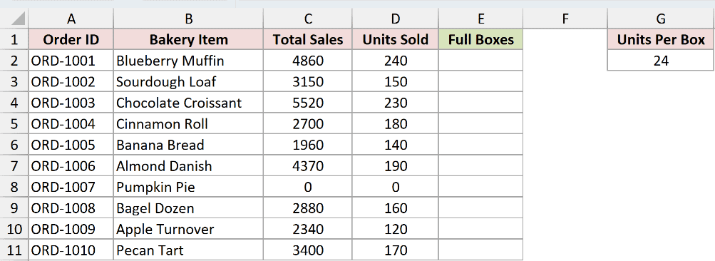
Here is the formula:

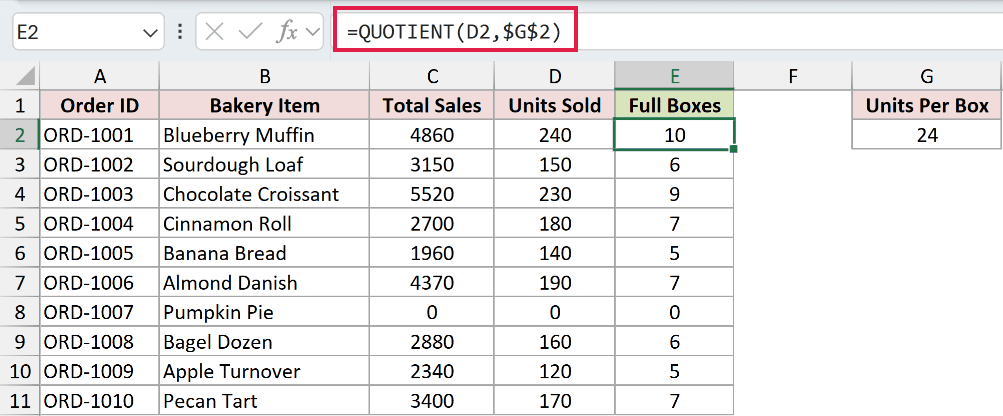
=QUOTIENT(D2,$G$2)

How does this formula work?

QUOTIENT takes two arguments, the number you’re dividing and the number you’re dividing by. It runs the division and then cuts off the remainder.

So 150 units divided by 24 is 6.25, and QUOTIENT reports 6. Six full boxes. Copy the formula down the column and you get 10, 6, 9, 7, 5, 7, 0, 6, 5 and 7.

Note that QUOTIENT cuts, it does not round. 190 divided by 24 is 7.917, which rounds to 8, but QUOTIENT still says 7. That’s the right answer for boxes and the wrong answer if you actually wanted rounding.

Note: QUOTIENT cuts toward zero, so a negative result behaves the way you might not expect. =QUOTIENT(-10,3) gives -3, not -4. Also, feed it text and you get a #VALUE! error rather than a division error.

Method #4: Using the MOD Function

QUOTIENT told you how many full boxes you get. MOD tells you what’s rattling around loose at the bottom.

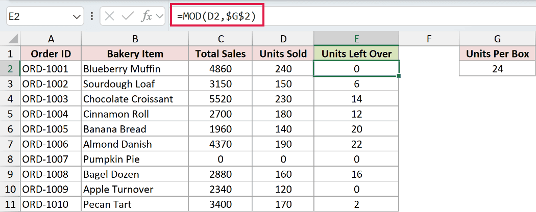
Below I have the same bakery data, with the box size of 24 in cell G2. Now I want the units left over after the full boxes are packed.

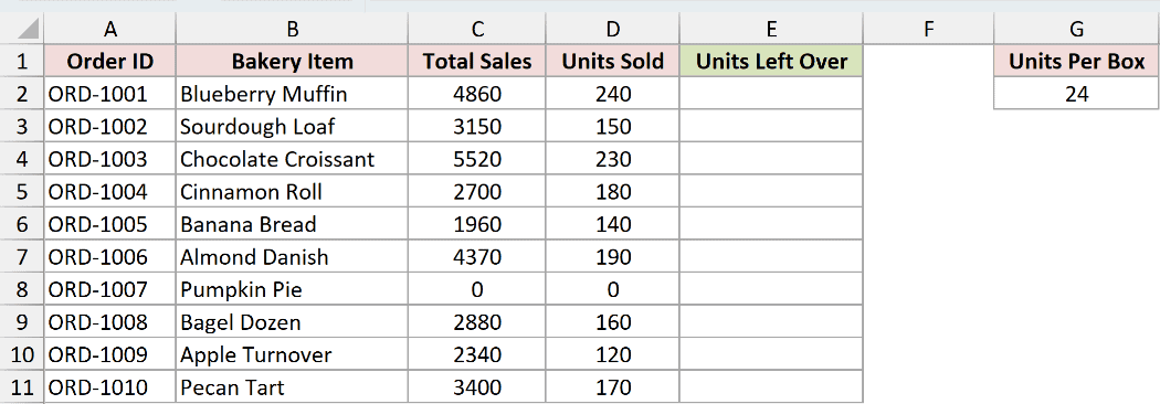
Here is the formula:

=MOD(D2,$G$2)

How does this formula work?

The MOD function divides the first number by the second and returns the remainder instead of the answer.

150 units divided by 24 gives 6 full boxes with 6 units spare, so MOD returns 6. Copy it down and you get 0, 6, 14, 12, 20, 22, 0, 16, 0 and 2.

Put Method #3 and Method #4 side by side and you have the full picture. The Sourdough Loaf order is 6 boxes plus 6 loose, and the Chocolate Croissant order is 9 boxes plus 14 loose.

Multiply the boxes back by 24, add the remainder, and you land on the original count every time.

Method #5: Using Paste Special (No Formula Needed)

If you’d rather not leave a formula behind, this one is for you. Paste Special rewrites the numbers where they sit.

Below I have the same bakery data. The sales figures in column C are in dollars and I want them in thousands, so every number needs dividing by 1000, in place, with no extra column.

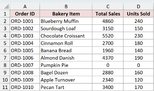
Here are the steps to divide the sales figures using Paste Special:

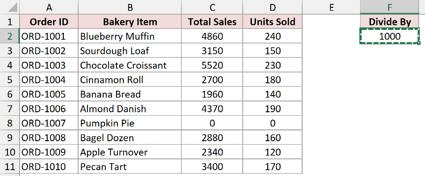
1. Type 1000 into any empty cell. I used F2. Select that cell and press Control + C to copy it.

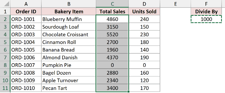
2. Select the numbers you want to divide, which is C2:C11 here.

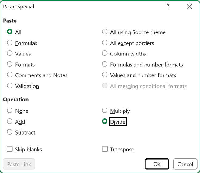
3. Press Control + Alt + V to open the Paste Special dialog box, then pick Divide under Operation. On a Mac it’s Command + Control + V.

4. Click OK.

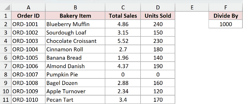
5. Delete the 1000 from F2. You’re done with it.

The sales column now reads 4.86, 3.15, 5.52, 2.7, 1.96, 4.37, 0, 2.88, 2.34 and 3.4.

This is a one-way trip. There’s no formula sitting there, so if the original sales figures ever change, nothing recalculates and you have to run the whole thing again.

Note: Paste Special overwrites whatever was in the cells you selected, and there is no way back once you’ve saved. Work on a copy of the column if you might want the original numbers again.

Method #6: Using IFERROR to Skip #DIV/0! Errors

Look back at row 7 in Method #1. The Pumpkin Pie hasn’t sold yet, so Excel is being asked to divide by zero and it answers with a #DIV/0! error.

Below I have the same bakery data. I want the price per unit again, but I want the untouched rows to stay blank instead of shouting at me.

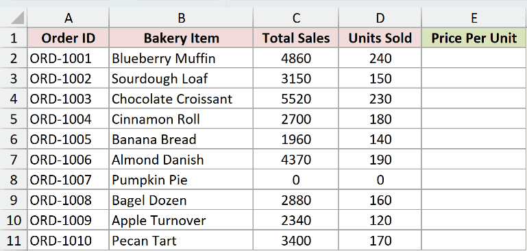
Here is the formula:

=IFERROR(C2:C11/D2:D11,"")

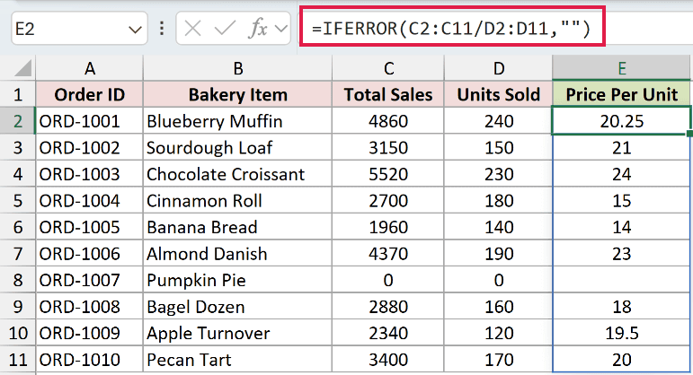
How does this formula work?

The IFERROR function runs the division first. If it works, you get the number. If it blows up, you get whatever you put in the second argument, which is an empty string here.

Swap the "" for a 0 or for "Not sold yet" if a blank looks too much like a mistake.

IFERROR hides every error, though, not just the division one. If a divisor cell has text in it instead of a number, that gets swallowed too and you’ll never know the data was wrong.

Note: The range version above needs Excel for Microsoft 365 or Excel 2021. On an older version, put =IFERROR(C2/D2,””) in E2 and copy it down the column.

Method #7: Using Power Query

If your data gets refreshed every week and you’re tired of redoing the same division, Power Query records the step once and replays it.

Below I have the same bakery data. I want a price per unit column, built by Power Query and loaded onto a fresh sheet.

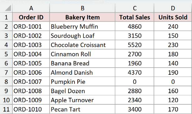
Here are the steps to divide two columns using Power Query:

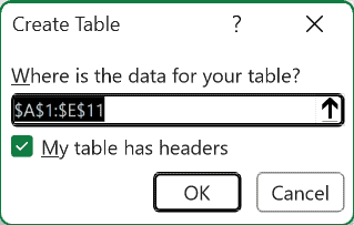
1. Click any cell in the data and press Control + T to turn it into an Excel Table, then click OK. Power Query won’t see your data until it’s a Table.

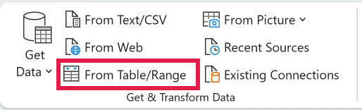
2. On the Data tab, click From Table/Range. The Power Query Editor opens.

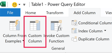
3. On the Add Column tab, click Custom Column.

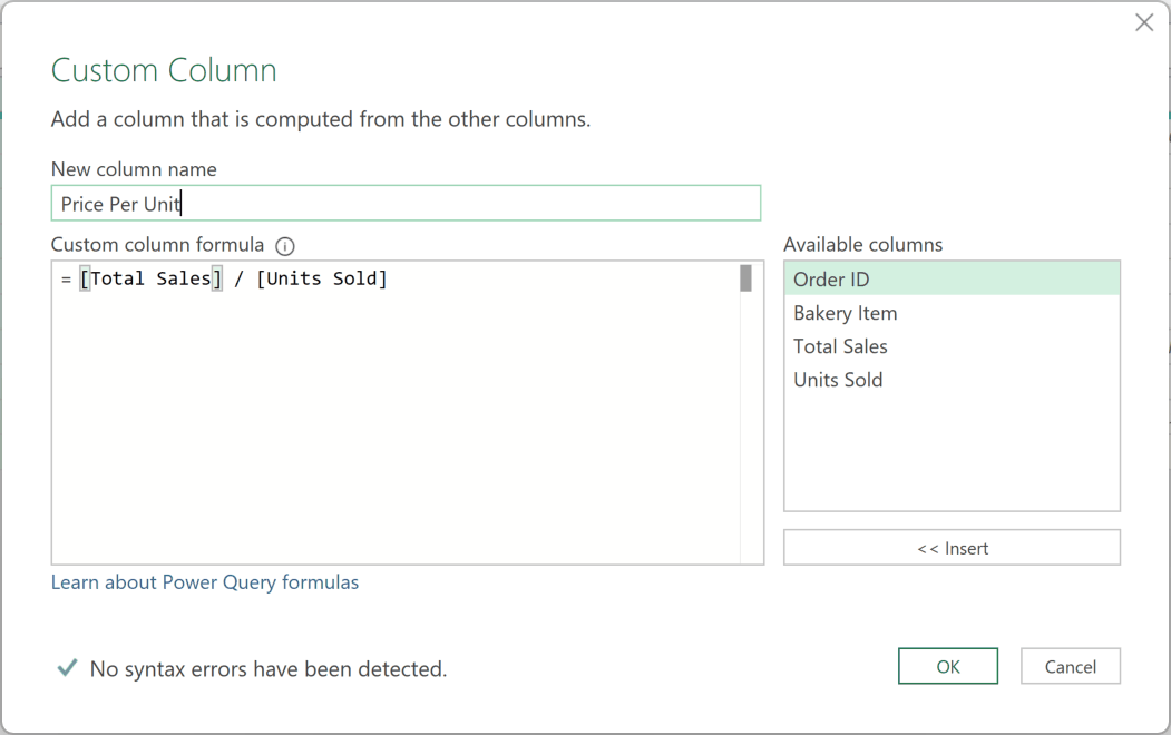
4. Type Price Per Unit in the New column name box. In the Custom column formula box, enter [Total Sales] / [Units Sold] and click OK.

5. On the Home tab, click Close & Load.

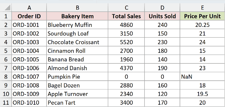
Power Query puts the result on a new worksheet as its own table. Your original data is untouched.

That’s the same forward slash from Method #1. The only thing that changes inside Power Query is how you point at the columns, in square brackets by name instead of by cell address.

Check the new column header once it appears. If it shows an Any icon, click it and pick Decimal Number so the results are treated as numbers rather than text.

When the sales numbers change, this does not update by itself. Go to the Data tab and click Refresh All, and Power Query replays every step on the new numbers.

Note: Power Query has no #DIV/0!. The Pumpkin Pie row divides zero by zero and comes back as NaN, which is Power Query’s way of saying the answer is not a number. Filter that row out before you divide.

For whole boxes instead of an exact price, type the following into that same formula box. It’s the Power Query equivalent of QUOTIENT.

Number.IntegerDivide([Units Sold], 24)

Method #8: Using a VBA Macro

If the same division lands on your desk every month on a freshly exported sheet, a macro turns it into one click.

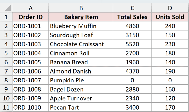
Below I have the same bakery data. I want to select the sales figures in column C and divide all of them by 1000 in one go.

Here is the VBA code:

Sub DivideSelection()

    Dim cell As Range
    Dim divisor As Double

    divisor = 1000

    If divisor = 0 Then
        MsgBox "You cannot divide by zero."
        Exit Sub
    End If

    For Each cell In Selection
        If Not IsEmpty(cell.Value) Then
            If IsNumeric(cell.Value) Then
                cell.Value = cell.Value / divisor
            End If
        End If
    Next cell

End Sub

Sub DivideSelection()

    Dim cell As Range
    Dim divisor As Double

    divisor = 1000

    If divisor = 0 Then
        MsgBox "You cannot divide by zero."
        Exit Sub
    End If

    For Each cell In Selection
        If Not IsEmpty(cell.Value) Then
            If IsNumeric(cell.Value) Then
                cell.Value = cell.Value / divisor
            End If
        End If
    Next cell

End Sub

Here are the steps to use this macro:

1. Select the cells you want to divide, which is C2:C11 here.
2. Press Alt + F11 to open the VBA Editor.
3. Go to Insert, then Module.
4. Paste the code above into the module.
5. Press F5 to run it.

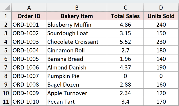
The macro walks through every cell you selected. It skips the empty ones, skips anything that isn’t a number, and divides the rest by whatever you set the divisor to.

Change the divisor = 1000 line to change the number you’re dividing by. The zero check above it stops the macro dead rather than filling your sheet with errors.

Note: There is no undo once a macro has run, so save first. If any selected cells hold formulas, the macro replaces them with plain numbers. Save the workbook as .xlsm if you want to keep the code.

Additional Notes About Dividing in Excel

• There is no divide sign in Excel. The ÷ symbol can be typed into a cell as text, but it won’t calculate anything. The forward slash is the only thing Excel treats as division.
• Type a slash as the very first character in a cell and Excel pops up the ribbon shortcut letters instead of typing a slash. That’s a leftover from Lotus 1-2-3. Start with an equals sign and it goes away.
• Division beats addition in Excel’s running order. =C2+C3/D2+D3 gives 5023.125 on my data, which is nonsense. =(C2+C3)/(D2+D3) gives about 20.54, which is the average price I actually wanted. Use brackets whenever you mix them.
• A blank divisor cell counts as a zero, so it throws the same #DIV/0! error a real zero does. A divisor cell with text in it throws a #VALUE! error instead.
• Showing fewer decimals does not round the number. The full value is still sitting in the cell, which is why a column of neatly displayed prices can add up to something slightly off.
• “Divide a cell” usually means chopping text apart, not arithmetic. That’s a different job, and it’s covered in splitting one column into multiple columns.

Frequently Asked Questions

Is there a DIVIDE function in Excel?

No. Excel gives you SUM for adding and PRODUCT for multiplying, but division only has the forward slash operator. QUOTIENT is the closest thing, and it only returns whole numbers.

If you’ve seen DIVIDE somewhere, that was Power BI, which uses a different formula language.

What is the division symbol in Excel?

The forward slash, /. It sits above the question mark on most keyboards and on the number pad. The ÷ symbol from maths class does nothing in an Excel formula.

How do I divide two columns and show the result as a percentage?

Divide as normal, then change the format. To see what share of total units the Blueberry Muffin order was, =D2/SUM(D2:D11) gives 0.1519. Press Control + Shift + % and it becomes 15%. Add two decimal places and you get 15.19%.

Why does my division result show as a date?

Because the cell you typed the formula into was already formatted as a date, and a formula doesn’t reset the cell’s format.

This catches people out most often when they insert a column next to a column of dates, since the new column picks up the date formatting.

Select the cell, go to the Home tab, and set the number format back to General or Number.

How do I round the result of a division?

Wrap the division in ROUND. =ROUND(C2/D2,0) turns the Apple Turnover’s 19.5 into 20, and the second argument is how many decimal places you want to keep.

The ROUND function changes the stored value, unlike the decimal buttons on the ribbon, which only change what you see.

Conclusion

For almost everything, the forward slash is all you need, and the range version of it fills a whole column without any dragging.

Reach for QUOTIENT and MOD when you want whole units and leftovers instead of decimals, and for Paste Special when you want no formula left sitting there. Power Query and the macro are for the jobs that come back every month.

Once you’ve got division sorted, the same logic runs the other way round in the multiplication formula.

Other Excel articles you may also like:

• How to Calculate Ratio in Excel? (4 Simple Ways)
• Convert Number of Days to Weeks in Excel
• Convert Days to Months in Excel
• Using MOD Operator in VBA
• How to Sum a Column in Excel?
• How to Subtract Multiple Cells from One Cell in Excel
• Round Up to the Nearest Whole Number in Excel (Formulas)