How to Combine Cells in Excel

If you want to pull the contents of a few cells into one cell, Excel’s Merge & Center button won’t do it. It squashes them into one big cell and keeps only the top-left value.

But nothing to worry about. Combining what’s actually inside the cells is easy once you know which route to take, and in this article I’ll show you seven ways to do it.

Combining Cells vs Merging Cells in Excel

These two sound like the same thing, and mixing them up is the reason a lot of people lose data.

Merging changes the layout. Excel takes the cells you selected, turns them into one big cell, and quietly deletes everything except the value in the top-left corner.

Combining changes the value. The cells stay exactly where they are, and you get a new cell holding all of their contents joined together.

So if your goal is a wider header stretching across four columns, you want merging, and it’s worth reading up on how to merge cells without losing data first.

If your goal is one cell holding the text from several cells, everything below is what you’re after.

Method #1: Using the Ampersand (&) Operator

The ampersand is the simplest way to stick cell contents together, and it works in every version of Excel ever made.

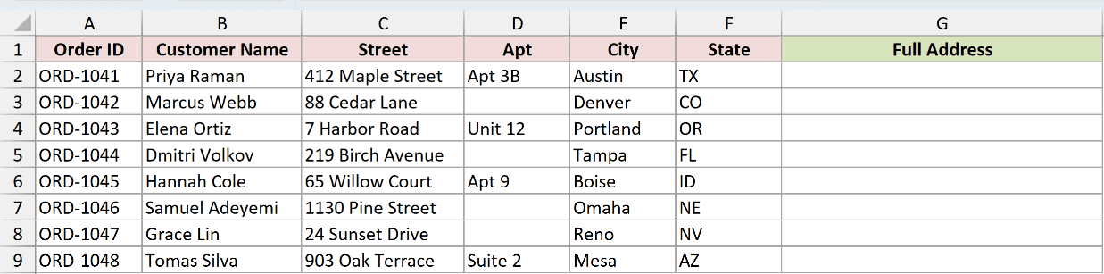
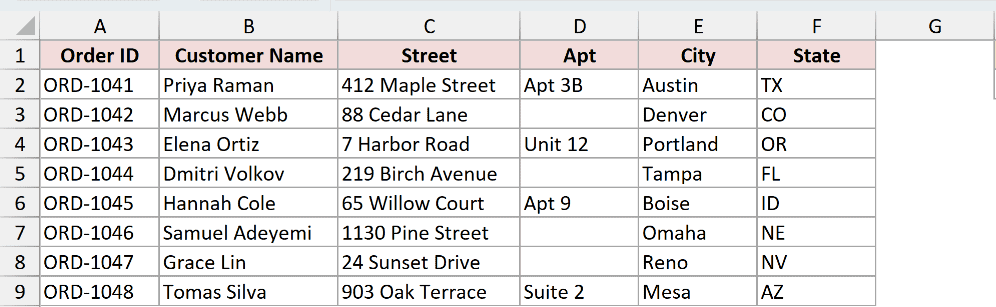
Below I have a dataset of customer orders, where the street, apartment, city and state each sit in their own column. I want to pull all four into a single full address in column G.

Here is the formula:

=C2&", "&D2&", "&E2&", "&F2

Enter it in cell G2 and copy it down the column.

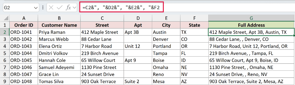
How does this formula work?

The ampersand is glue. It takes whatever is on its left, whatever is on its right, and returns them as one piece of text.

Everything in quotes is text I typed in myself. ", " is a comma followed by a space, and I need one of those between every pair of cells, which is why the formula has three of them.

If you’re on Microsoft 365, you can point the same formula at whole columns instead and it spills down the column automatically:

=C2:C9&", "&D2:D9&", "&E2:E9&", "&F2:F9

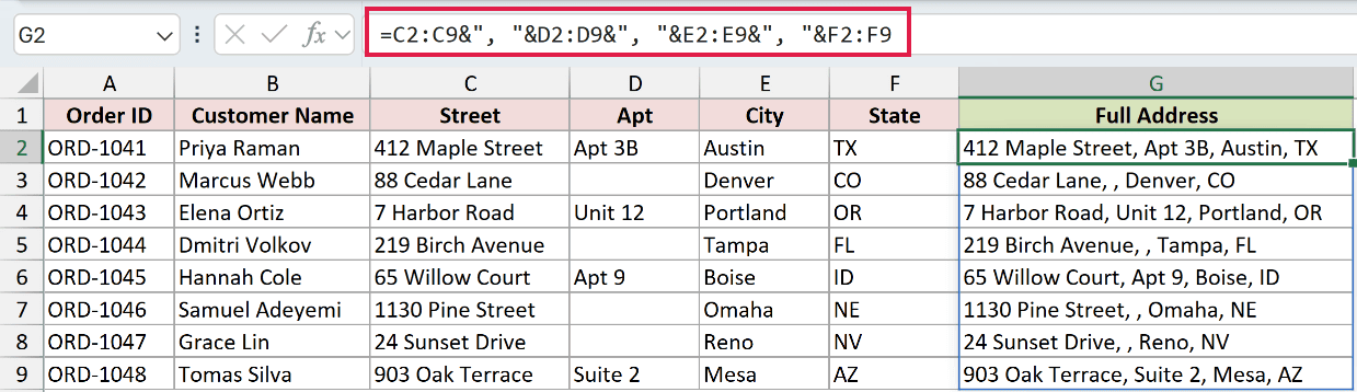
Note: Rows where the Apt column is empty come out with two commas in a row, like 88 Cedar Lane, , Denver, CO. The ampersand adds every separator you type, whether or not there is anything sitting on either side of it. Method #3 is the one that fixes this.

Method #2: Using the CONCAT Function

Here’s another way to do the same thing, and this one can swallow a whole range in one go instead of making you name every cell.

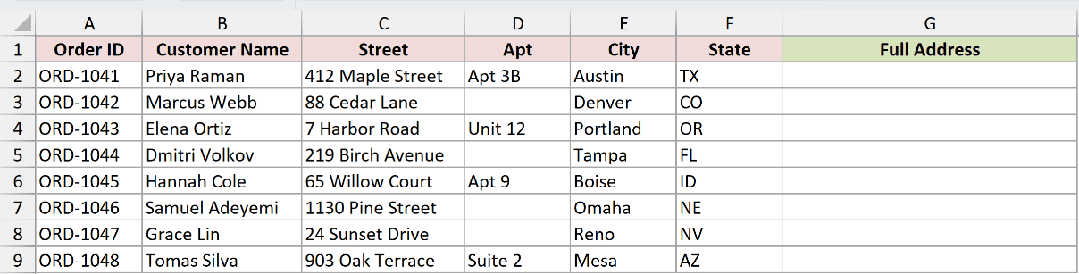
Below I have the same order dataset, with the street, apartment, city and state in separate columns, and I want them combined into column G.

Here is the formula:

=CONCAT(C2:F2)

Enter it in cell G2 and copy it down the column.

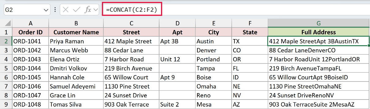
That gives you 412 Maple StreetApt 3BAustinTX, which is probably not what you had in mind.

CONCAT happily takes a range, but it has no separator argument at all. It jams the values together exactly as they are.

To get the commas back, you have to hand them to CONCAT as arguments of their own:

=CONCAT(C2,", ",D2,", ",E2,", ",F2)

Again, enter it in cell G2 and copy it down.

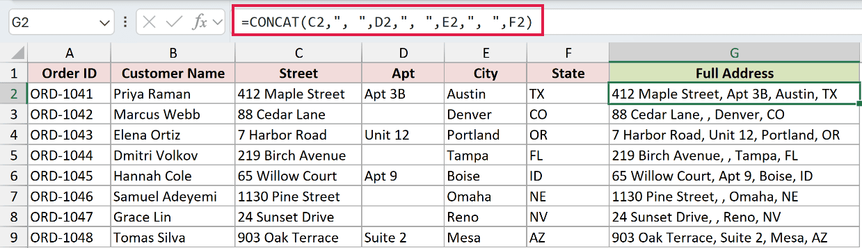
How does this formula work?

CONCAT reads its arguments left to right and returns them as one string. Cell references bring in cell values, and anything in quotes goes in literally.

So the range version is great when you want the values run together, and the long version is what you use when you need something between them. Either way, blank cells still leave you with a stray comma.

Note: The CONCAT function needs Excel 2019 or a Microsoft 365 subscription. Excel 2016 only has it with a subscription, and on anything older you will get a #NAME? error, so the CONCATENATE function is the one to use instead. It behaves the same way, except it cannot take a range, so you have to list every cell separately.

Method #3: Using the TEXTJOIN Function

If you’re combining more than two or three cells, this is the one I’d reach for. You type the separator once and it handles the rest.

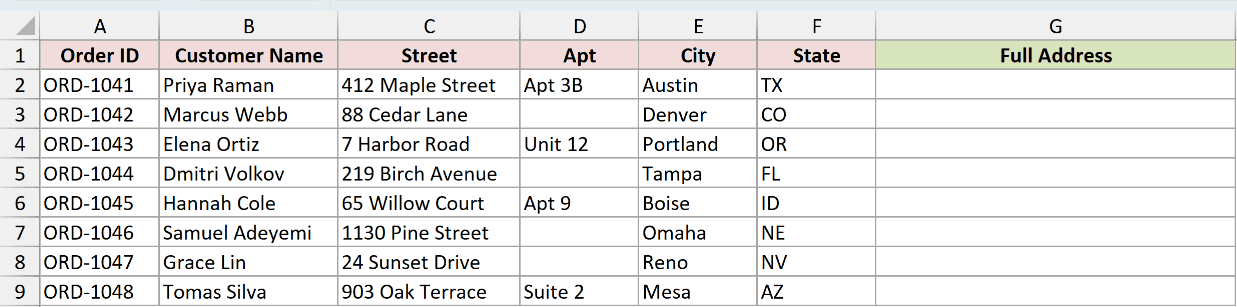
Below I have the same order dataset. This time I want the full address in column G, and I want the rows with an empty Apt column to come out clean.

Here is the formula:

=TEXTJOIN(", ",TRUE,C2:F2)

Enter it in cell G2 and copy it down the column.

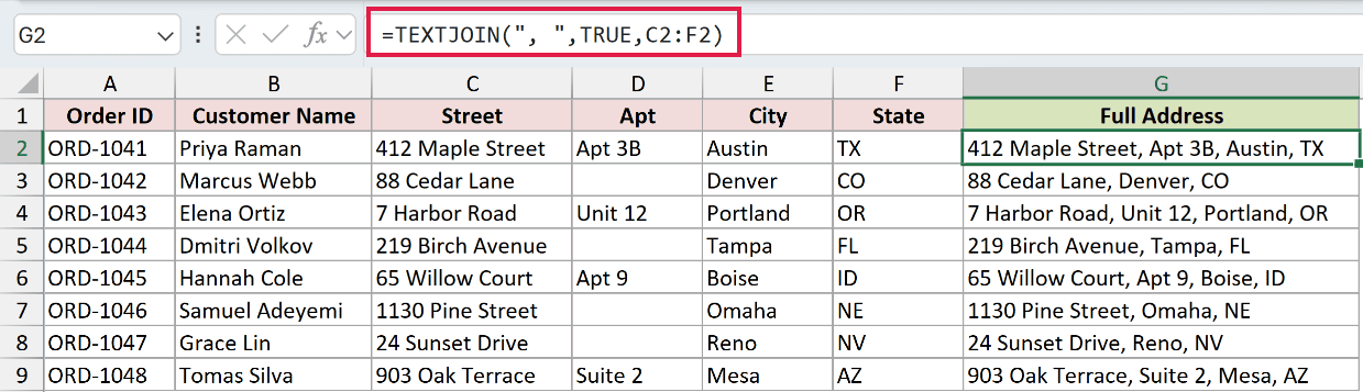
How does this formula work?

The first argument, ", ", is the separator. TEXTJOIN drops it between every pair of values so you never type it more than once.

The second argument is the one that matters here. TRUE tells TEXTJOIN to ignore empty cells, so Marcus Webb’s row comes back as 88 Cedar Lane, Denver, CO instead of carrying a gap where the Apt value should have been.

The third argument is just the range you want joined.

TEXTJOIN also handles the other direction. Point it at a single column and you get every value in that column inside one cell:

=TEXTJOIN(", ",TRUE,B2:B9)

This one goes in a single empty cell. There is nothing to copy down, because the whole column collapses into that one result.

That returns all eight customer names as one comma-separated line, which is handy when you need to paste a list somewhere outside Excel.

Note: The TEXTJOIN function takes up to 252 arguments, and a range counts as one of them. If the finished string runs past 32,767 characters, which is the most a single cell can hold, you get a #VALUE! error instead of a result.

Method #4: Using the Fill Justify Feature

If you’d rather not write a formula at all, Excel can push a column of text into the top cell for you.

Fill Justify works on one column at a time and only on text. Point it at numbers or formulas and Excel refuses with “Cannot justify cells containing numbers or formulas.” That makes it best for short text values, so I’ll use the State column here.

Below I have the same order dataset, and I want all eight state codes sitting in cell F2.

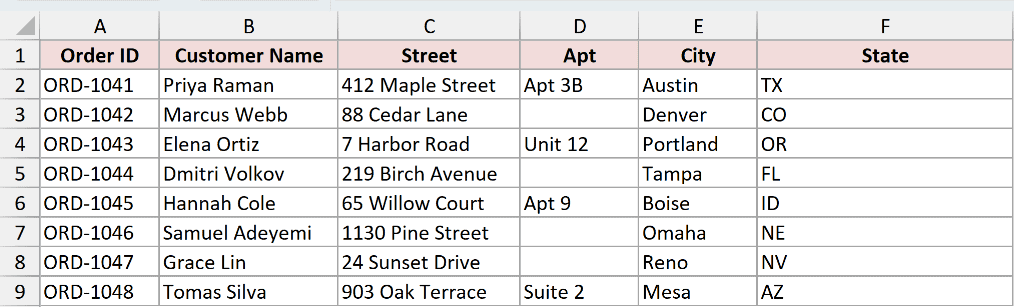
One thing to do first: Justify reflows the text into as many rows as it needs, and it overwrites whatever is sitting below your selection without asking. Make sure the space underneath is empty.

Here are the steps to combine the cells with Fill Justify:

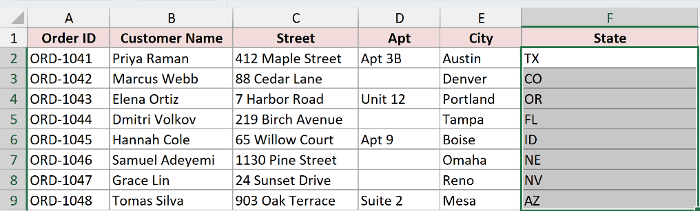
1. Widen column F so there is room for the whole finished string, then select the range F2:F9.

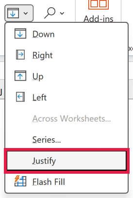
2. On the Home tab, click Fill in the Editing group, then click Justify.

Excel reflows the whole column of text to fit the width you set, so TX CO OR FL ID NE NV AZ ends up in F2 and the cells below it are cleared.

Notice that Fill Justify separates the values with spaces. There is no way to ask it for commas.

Note: A justified cell holds at most 255 characters. Longer text flows on into the cells below, but if a single word is longer than that on its own, Excel cuts it off at 255 and the rest is gone.

Method #5: Using the Flash Fill Feature

Flash Fill watches what you type, works out the pattern, and finishes the column for you.

Below I have the same order dataset. This time I’m combining the street, city and state, and leaving the Apt column out of it, because the blank cells in that column confuse Flash Fill’s pattern detection.

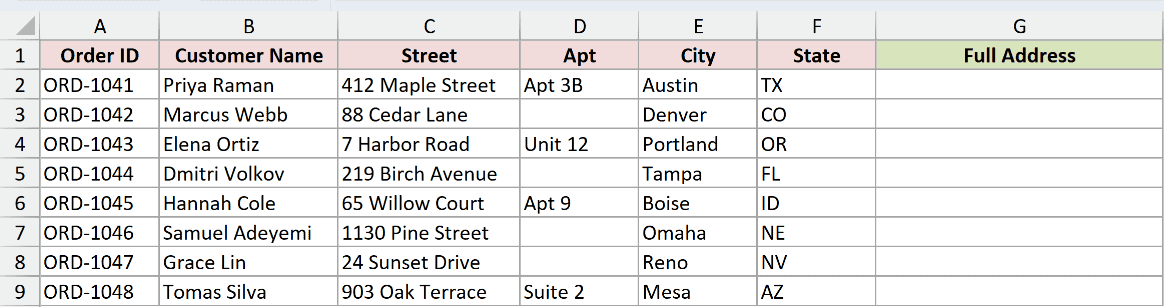
Here are the steps to combine the cells with Flash Fill:

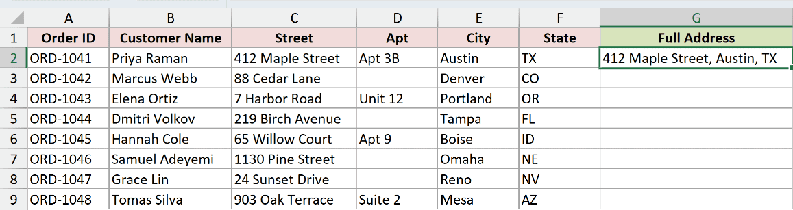
1. In cell G2, type the finished address by hand: 412 Maple Street, Austin, TX

2. Select the range G2:G9 and press Ctrl + E.

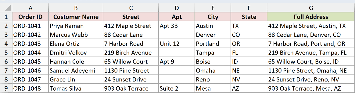
Excel matches what you typed against the columns beside it, spots that you took the street, the city and the state in that order, and fills the rest of the column the same way.

What you get is a one-time fill, not a formula. Fix a typo in the Street column later and the combined column will sit there showing the old text.

Note: Flash Fill needs Excel 2013 or later, and Ctrl + E is the Windows shortcut. On a Mac you pick Flash Fill from the Data menu instead.

Method #6: Using Power Query Merge Columns

If this is something you do every time a new file lands on your desk, Power Query is worth the extra few clicks. You set it up once and refresh it after that.

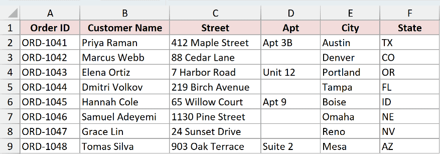
Below I have the same order dataset, and I want a Full Address column built from the street, apartment, city and state.

Here are the steps to combine the cells with Power Query:

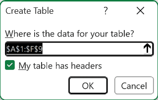
1. Click any cell inside the data and press Ctrl + T to turn it into an Excel Table, then click OK. Power Query cannot see a plain range, so this step is not optional.

2. With a cell in the Table selected, go to the Data tab and click From Table/Range. The Power Query Editor opens with your data in it.

3. Click the Street column header, then hold Ctrl and click Apt, City and State. Click them in the order you want them combined, because that is the order Power Query uses.

4. Go to the Add Column tab and click Merge Columns. In the dialog, set Separator to Custom, type a comma followed by a space, name the new column Full Address, and click OK.

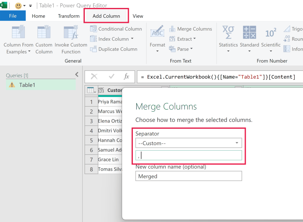
Use Merge Columns on the Add Column tab, not the one on the Transform tab. The Transform version replaces your four original columns with the combined one and you lose them.

It also handles the empty cells differently. The Add Column version skips a blank Apt the way TEXTJOIN does, so Marcus Webb’s row comes back as 88 Cedar Lane, Denver, CO.

The Transform version leaves the gap in and you get 88 Cedar Lane, , Denver, CO.

5. On the Home tab, click Close & Load.

Power Query drops the result onto a brand new sheet as its own table. Your original data is untouched, which catches people out the first time.

Note: Power Query does not refresh on its own. When the source data changes, go to the Data tab and click Refresh All, otherwise the loaded table keeps showing yesterday’s addresses.

Method #7: Using a VBA User Defined Function

If you’re stuck on Excel 2016 or older, TEXTJOIN isn’t there. You can build your own version in about ten lines of VBA and then use it like any other function.

Below I have the same order dataset, and I want a function I can point at any range to get its contents back as one string.

Here is the VBA code:

Function JoinCells(rng As Range, Optional delim As String = ", ") As String
    Dim c As Range
    Dim result As String
    For Each c In rng
        If Len(Trim(c.Value)) > 0 Then
            If Len(result) > 0 Then result = result & delim
            result = result & c.Value
        End If
    Next c
    JoinCells = result
End Function

Function JoinCells(rng As Range, Optional delim As String = ", ") As String
    Dim c As Range
    Dim result As String
    For Each c In rng
        If Len(Trim(c.Value)) > 0 Then
            If Len(result) > 0 Then result = result & delim
            result = result & c.Value
        End If
    Next c
    JoinCells = result
End Function

Here are the steps to use this function:

1. Press Alt + F11 to open the VBA Editor
2. Insert a new module (Insert → Module)
3. Paste the code above into the module
4. Press Alt + Q to go back to Excel

Now you can use it on the worksheet like anything built in:

=JoinCells(B2:B9)

The loop walks through every cell in the range you gave it. Len(Trim(c.Value)) > 0 skips anything blank, so you never get a stray separator, and the separator only goes in when there is already something in the result.

The second argument is optional. Leave it out and you get commas, or pass your own with =JoinCells(C2:F2," - ").

Note: Save the file as a macro-enabled workbook (.xlsm) or the code disappears the moment you close it. Anyone you send the file to needs macros enabled as well, so this is not the method to use for something you are emailing around.

Additional Notes About Combining Cells in Excel

• The combined cell holds a formula, not text, so deleting the source columns breaks every result. Copy the results column, right-click and choose Paste Special, then Values, before you clear anything out.
• Numbers and dates lose their formatting when you combine them. A date turns back into the serial number Excel stores underneath, so 01-Aug-2026 shows up as something like 46235. Wrap it in TEXT to keep the format you want.
• Put the space inside the separator. Type ", " rather than ",". Relying on trailing spaces already sitting in your data is how you end up with addresses that look almost right.
• A cell tops out at 32,767 characters, and TEXTJOIN and CONCAT both return a #VALUE! error past that. Fill Justify is stricter still, capping each justified cell at 255.

Frequently Asked Questions

Why does my combined date turn into a number like 46235?

Excel stores dates as serial numbers and only shows them as dates because of the cell’s formatting. Combining strips that formatting away and you see the raw number.

Wrap the cell in TEXT to fix it, like =TEXTJOIN(", ",TRUE,B2,TEXT(H2,"dd-mmm-yyyy")). There’s more on this in the guide to combining date and time.

How do I keep the combined text after I delete the original columns?

Select the column with your results, press Ctrl + C, then right-click and choose Paste Special followed by Values. That swaps the formulas for plain text, and the source columns are then safe to delete.

Why do CONCAT and TEXTJOIN give me a #NAME? error?

Your version of Excel doesn’t have them. Both arrived with Excel 2019, and Excel 2016 only gets them with a Microsoft 365 subscription. Use the ampersand operator from Method #1 instead, which works everywhere.

How do I put a line break between the combined cells instead of a comma?

Use CHAR(10) as the separator, so =TEXTJOIN(CHAR(10),TRUE,C2:F2), and then turn on Wrap Text for that cell or nothing will look any different. The full walkthrough is in how to concatenate with line breaks.

Is there a limit to how many cells I can combine into one cell?

TEXTJOIN and CONCAT take up to 252 arguments, and a whole range only counts as one of them, so the argument limit is rarely what stops you. The real ceiling is the cell itself at 32,767 characters.

Conclusion

Combining cells comes down to what you’re joining and what you’ve got installed. TEXTJOIN is the one I use most, because you type the separator once and it skips blanks without being asked.

It also works the same way whether you point it at a row of cells or a whole column.

If you’re on an older version, the ampersand operator does the same job with a bit more typing. And if the data keeps changing, set it up in Power Query once and refresh it from then on.

Other Excel articles you may also like:

• How to Combine Two Columns in Excel (with Space/Comma)
• How to Merge First and Last Name in Excel?
• Concatenate in Power Query (Columns, Text, Numbers)
• How to Add Comma Between Names in Excel
• How to Add Text to the Beginning or End of all Cells in Excel
• Opposite of Concatenate in Excel (Reverse Concatenate)
• Table.CombineColumns Function (Power Query M)
• How to Split One Column into Multiple Columns in Excel