How to Insert Page Breaks in Excel (5 Easy Ways)

If you want to control exactly where your Excel sheet splits when you print it, you can’t just hit Enter and hope for the best. Excel decides where the pages break on its own, based on your margins, scale and paper size.

But nothing to worry about. You can put a break exactly where you want it, and in this article I’ll show you five ways to insert a page break in Excel.

Table of Contents

Method #1: Using the Page Layout Breaks Menu

This is the one to learn first. It works from any view, and it puts the break exactly where you ask for it.

Below I have a sales order dataset with 12 orders grouped by region, and I want each region to start on a fresh printed page.

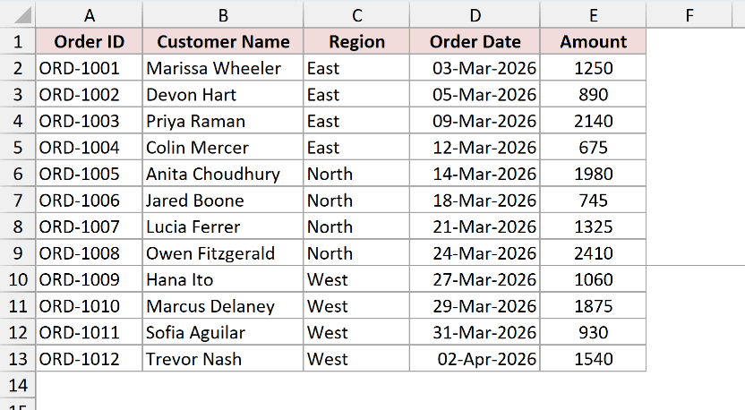
The manual page break line between rows 9 and 10, sending everything below to a new page

The trick is knowing what to select before you click. A horizontal page break splits the sheet top to bottom, so you select the row below where you want the split. The break lands just above whatever you selected.

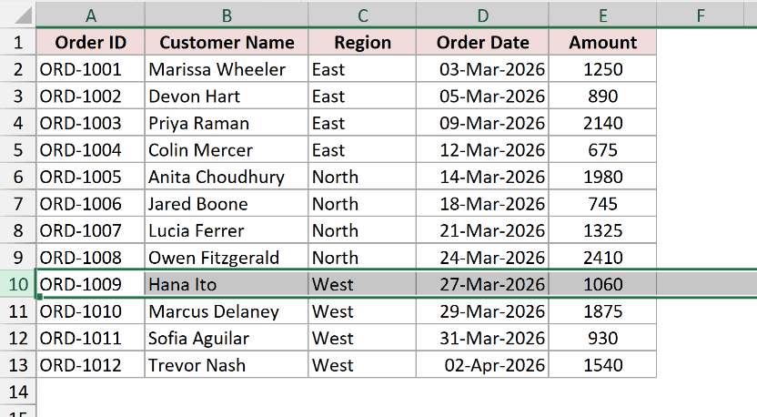
In my data the West orders start in row 10, so row 10 is what I select.

Here are the steps to insert a horizontal page break:

Click the row header for row 10 to select the whole row.

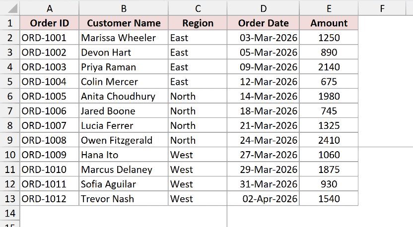
Both break lines from a single cell selection, one above row 10 and one left of column D

On the Page Layout tab, in the Page Setup group, click Breaks, then click Insert Page Break.

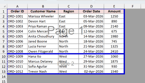
Page Break Preview with a dashed automatic break and a solid manual break over the greyed layout

A line now sits between row 9 and row 10. Everything from row 10 down prints on a new page.

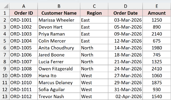
Sales orders dataset grouped by region, where each region should print on its own page

A vertical page break works the same way, just rotated. It splits the sheet left to right, so you select the column to the right of where you want the split, and the break lands to the left of it.

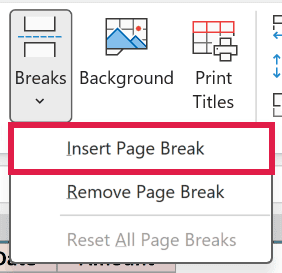
I want Order Date and Amount on their own page, so I select column D.

Here are the steps to insert a vertical page break:

Click the column header for column D to select the whole column.

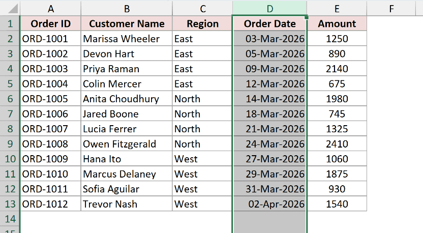
Row 10 selected, the row below where the horizontal page break should land

On the Page Layout tab, click Breaks, then click Insert Page Break.

The Breaks dropdown on the Page Layout tab with the Insert Page Break command

If you select a single cell instead of a whole row or column, Excel gives you both breaks at once, one above the cell and one to its left.

Select cell D10 and run the same command, and you get a horizontal break above row 10 plus a vertical break to the left of column D.

Column D selected, the column to the right of where the vertical page break should land

That’s usually the reason a break shows up somewhere you didn’t ask for. You had a cell selected, not a row.

Note: If nothing seems to happen when you insert a break, check Page Layout > Scale to Fit. When Width or Height is set to 1 page, Excel squeezes everything onto that page and ignores your manual breaks. Set both back to Automatic and the break shows up.

Method #2: Using the Alt + P + B + I Shortcut

Here’s the same command without the mouse. If you’re adding several breaks in one sitting, this saves a lot of clicking.

Below I have the same order dataset, and I want a break above row 10 again.

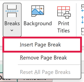
The same Breaks dropdown used to insert a vertical page break to the left of column D

Select row 10, then press these keys one after another (not together): Alt, then P, then B, then I.

Think of it as P for Page Layout, B for Breaks, I for Insert. Excel shows you the letter hints on the ribbon as you go, so you can watch it happen.

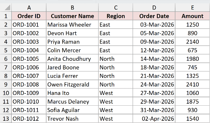
Sales orders dataset ready for the Alt P B I keyboard sequence

The same menu gives you two more sequences worth remembering. Alt + P + B + R removes the break your selection sits on, and Alt + P + B + A resets every manual break on the sheet.

Note: This is a Windows-only shortcut. It works by walking the ribbon with the Alt key, and Excel for Mac doesn’t have that system. On a Mac, use the Page Layout tab from Method #1.

Method #3: Using Page Break Preview

The first two methods place a break blind. You pick a row, you click, and you find out later whether the pages actually came out the way you wanted. Page Break Preview fixes that by showing you the whole layout at once.

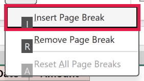
Below I have the same dataset, and this time I want to see where the pages fall before I commit to anything.

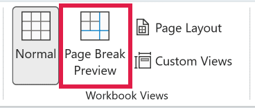
The ribbon key hints showing as the Breaks menu opens with Alt P B

Here are the steps to switch into Page Break Preview:

On the View tab, in the Workbook Views group, click Page Break Preview. You can also click the Page Break Preview icon on the status bar at the bottom right.

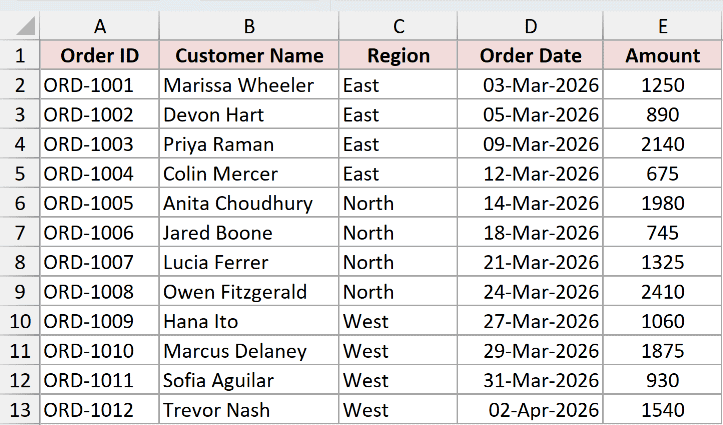
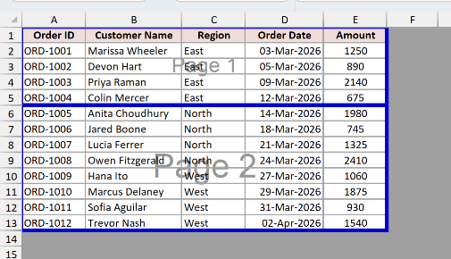
Sales orders dataset about to be viewed in Page Break Preview

Excel greys out everything outside the print area and stamps a big Page 1, Page 2 watermark on each chunk. The lines you see are colour coded:

Dashed blue lines are automatic breaks. Excel worked those out from your margins, scale and paper size.
Solid blue lines are manual breaks. Those are the ones you put there.

The Page Break Preview command in the Workbook Views group of the View tab

To place a break here, just drag a line. Hover over any break until the cursor turns into a double-headed arrow, then drag it to the row or column you want.

Drag one of the dashed automatic lines and it turns solid. Moving an automatic break converts it to a manual one, so it stops recalculating on you.

A dragged break line turned solid, converted from automatic to manual

You can also add a fresh break from the right-click menu while you’re in this view. Right-click the row header, column header or cell that sits below or to the right of where you want the split, then click Insert Page Break.

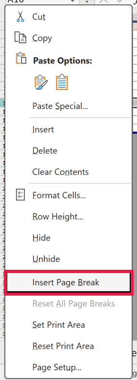
The right-click menu in Page Break Preview with the Insert Page Break command

That right-click menu is the fastest route when you’re placing four or five breaks in a row, since you never leave the sheet. When you’re done, switch back to Normal view from the View tab.

Note: If dragging does nothing, cell drag-and-drop is switched off. Go to File > Options > Advanced and tick “Enable fill handle and cell drag-and-drop”, then try again.

Method #4: Using Subtotal With Page Break Between Groups

Everything so far places one break at a time. If you want every region, department or month to start on its own page, that gets tedious fast.

Excel’s Subtotal command has a checkbox that does the whole job in one go.

Below I have the same order data, sorted by region, and I want each region on its own printed page with its own total.

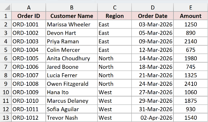
Sales orders sorted by region, ready for Subtotal to add totals and page breaks

Sorting first is not optional here. Subtotal walks down the column looking for the value to change, so if your regions are scattered you’ll get a break every few rows instead of three clean pages.

Here are the steps to insert a page break between each group:

Click any cell inside your data.
On the Data tab, in the Outline group, click Subtotal.

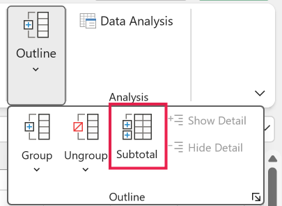
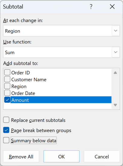
Excel ribbon showing the Outline menu with the Subtotal option highlighted by a red box

In the Subtotal dialog box, set “At each change in” to Region, set “Use function” to Sum, and tick Amount under “Add subtotal to”. Then tick the “Page break between groups” checkbox and click OK.

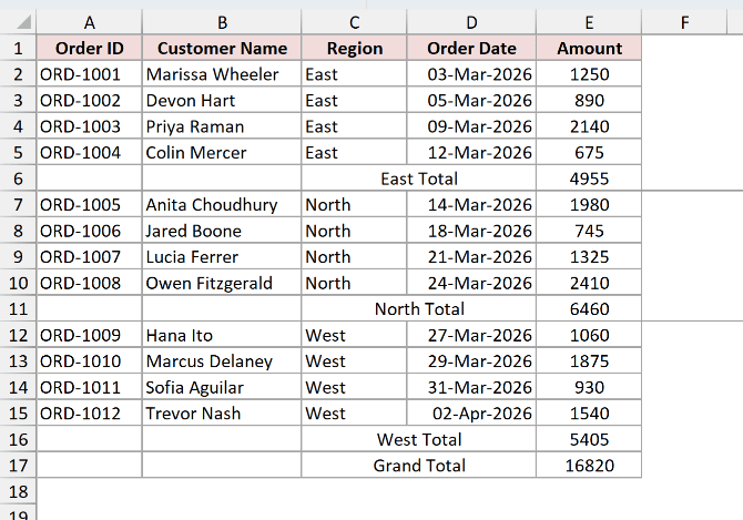
Subtotal dialog box set to sum Amount for each Region, with Page break between groups checked

Excel drops in a subtotal row after each region and a horizontal break right behind it. East totals 4955, North totals 6460, West totals 5405, and the grand total at the bottom is 16820.

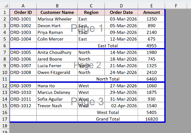
Subtotal rows added after each region with a page break line behind each one

Switch to Page Break Preview and you’ll see three regions on three pages, without placing a single break by hand.

Page Break Preview showing the three regions split across three pages

Note: Subtotal is greyed out if your data is formatted as an Excel Table. Click anywhere in the table, go to Table Design > Convert to Range, and the command wakes up.

Method #5: Using a VBA Macro

VBA earns its place when you’re dealing with hundreds of rows, or a report you rebuild every month and re-break every time.

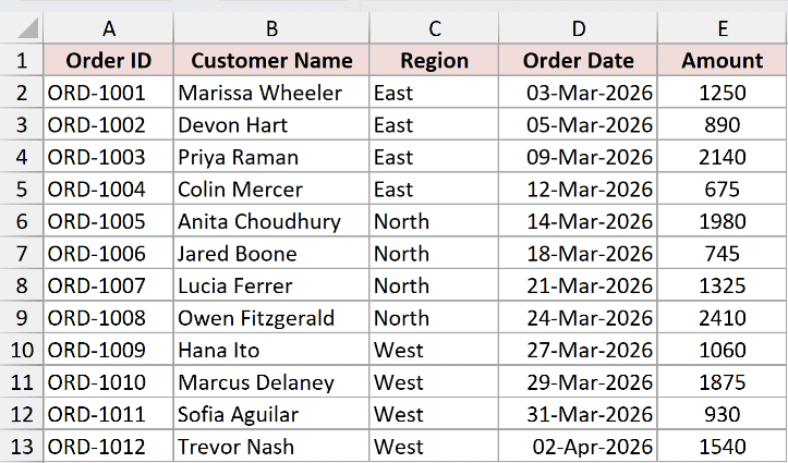
Below I have the same order dataset on a sheet named Orders.

The sales orders on a sheet named Orders, ready for the VBA page break macros

If you just want breaks at fixed positions, this is all it takes:

Sub InsertFixedPageBreaks()

    Dim ws As Worksheet
    Set ws = ThisWorkbook.Worksheets("Orders")

    ' Horizontal break above row 10
    ws.Rows(10).PageBreak = xlPageBreakManual

    ' Vertical break to the left of column D
    ws.Columns("D").PageBreak = xlPageBreakManual

End Sub

Sub InsertFixedPageBreaks()

    Dim ws As Worksheet
    Set ws = ThisWorkbook.Worksheets("Orders")

    ' Horizontal break above row 10
    ws.Rows(10).PageBreak = xlPageBreakManual

    ' Vertical break to the left of column D
    ws.Columns("D").PageBreak = xlPageBreakManual

End Sub

Setting PageBreak to xlPageBreakManual on a row gives you a horizontal break above it. Do the same on a column and you get a vertical break to its left. Swap in xlPageBreakNone and it clears that break instead.

The more useful version loops down the sheet and breaks every time the region changes, so it keeps working when you add rows next month:

Sub BreakOnRegionChange()

    Dim ws As Worksheet
    Dim lastRow As Long
    Dim i As Long

    Set ws = ThisWorkbook.Worksheets("Orders")
    lastRow = ws.Cells(ws.Rows.Count, "C").End(xlUp).Row

    ' Clear any manual breaks already on the sheet
    ws.ResetAllPageBreaks

    For i = 3 To lastRow
        If ws.Cells(i, "C").Value <> ws.Cells(i - 1, "C").Value Then
            ws.Rows(i).PageBreak = xlPageBreakManual
        End If
    Next i

End Sub

Sub BreakOnRegionChange()

    Dim ws As Worksheet
    Dim lastRow As Long
    Dim i As Long

    Set ws = ThisWorkbook.Worksheets("Orders")
    lastRow = ws.Cells(ws.Rows.Count, "C").End(xlUp).Row

    ' Clear any manual breaks already on the sheet
    ws.ResetAllPageBreaks

    For i = 3 To lastRow
        If ws.Cells(i, "C").Value <> ws.Cells(i - 1, "C").Value Then
            ws.Rows(i).PageBreak = xlPageBreakManual
        End If
    Next i

End Sub

Here are the steps to use this macro:

Press Alt + F11 to open the VBA Editor
Go to Insert, then Module
Paste the code above
Press F5 to run the macro

The loop starts at row 3 because it compares each row against the one above it, and row 2 has nothing above it but the header.

On my data the region changes at row 6 and row 10, so it drops in exactly two breaks and I end up with three pages.

If you ever want to check your work in code, ws.HPageBreaks.Count tells you how many horizontal breaks are on the sheet and ws.VPageBreaks.Count does the same for vertical ones.

Note: Save the workbook as a macro-enabled file (.xlsm) if you want to keep the code. A regular .xlsx quietly throws the macro away when you close it.

Additional Notes About Inserting Page Breaks in Excel

Scale to Fit beats your breaks. If Page Layout > Scale to Fit has Width or Height set to 1 page, every manual break gets ignored. This is far and away the most common reason a break “doesn’t work”. If you actually want everything on one sheet, that’s a job for fit to page instead.
A print area is not a page break. Setting a print area limits which cells print at all. A page break decides where the printed cells split. They’re different jobs and you’ll often want both.
Your headers won’t follow you. Once your data spans several pages, page 2 onwards prints with no column headings unless you set a row to print on every page using Print Titles.
Watch for [Group] in the title bar. If you have several sheet tabs selected, the break gets applied to all of them at once.
Removing a break is the mirror image of adding one. Select the row below or column to the right and use Page Layout > Breaks > Remove Page Break, or see the full walkthrough on how to remove page breaks in Excel.

Frequently Asked Questions

Why is my page break not working in Excel?

Nine times out of ten it’s the Scale to Fit setting. Go to the Page Layout tab and check the Width and Height boxes, and if either says “1 page”, change it back to Automatic.

Why do my page breaks move on their own?

Automatic breaks (the dashed ones) get recalculated whenever you change margins, paper size, orientation, scale, column widths or row heights. Manual breaks stay put.

If you want a break to stop drifting, drag it once in Page Break Preview and it converts to a manual break.

Will my header row repeat on every page after a page break?

Not automatically. Go to Page Layout > Print Titles and set “Rows to repeat at top” to your header row. Without it, only page 1 gets the column names.

Do page breaks apply when I save the sheet as a PDF?

Yes. Saving as PDF uses the same page setup as a normal printout, so your breaks decide where each PDF page ends. Add one horizontal break to a sheet that fits on a single page and the PDF comes out as two.

Conclusion

Page breaks look fiddly until you get the selection rule straight: pick the row below for a horizontal break, the column to the right for a vertical one, and a single cell if you want both.

For most sheets I’d switch to Page Break Preview first so I can see the layout, then use Page Layout > Breaks to place things exactly. And if you’re printing grouped data like sales by region, let Subtotal do the work for you.

Other Excel articles you may also like: