
If you want to find the largest value that meets one or more conditions, the MAXIFS function is what you’re looking for.
In this article, I’ll show you how to use MAXIFS with text, numbers, dates, wildcards, and multiple conditions.
MAXIFS returns one value, but it also works inside dynamic array formulas that evaluate several criteria at once.
MAXIFS Function Syntax in Excel
The MAXIFS syntax starts with the values to check, followed by one or more range-and-criterion pairs.
=MAXIFS(max_range, criteria_range1, criteria1, [criteria_range2, criteria2], ...)
max_range: The cells containing the values from which you want the maximum.criteria_range1: The first range Excel checks against your condition.criteria1: The condition applied tocriteria_range1.[criteria_range2, criteria2]: Optional additional range-and-condition pairs. You can add up to 126 pairs.
When to Use MAXIFS Function
- Find the highest sales value for a specific region, product, or employee.
- Return the largest value that satisfies several conditions at the same time.
- Work with comparison operators, dates, and wildcard text criteria.
- Find the latest date that meets your conditions. MAXIFS can compare dates because Excel stores them as numbers.
Example 1: Highest Value with One Criterion
Let’s start with a simple example.
Below is the dataset of property listings, with listing IDs, property types, and sale prices.
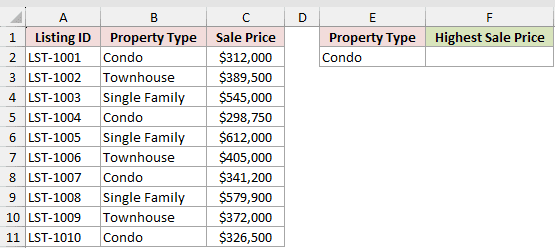
I want to find the highest sale price for the property type entered in cell E2.
Here is the formula:
=MAXIFS(C2:C11,B2:B11,E2)
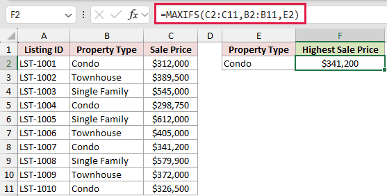
The formula checks property types in B2:B11 and returns the largest matching sale price from C2:C11.
Since E2 contains Condo, the result is $341,200.
Example 2: MAXIFS with Multiple Criteria
Here’s a practical two-condition example.
Below is the dataset of restaurant sales, with each location, shift, and daily sales amount.
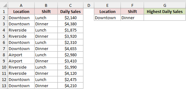
I want the highest daily sales for the Downtown location during the Dinner shift.
Here is the formula:
=MAXIFS(C2:C13,A2:A13,E2,B2:B13,F2)
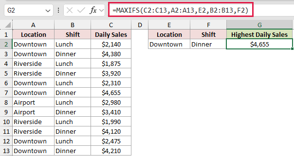
MAXIFS checks the location in A2:A13 and the shift in B2:B13. A row must satisfy both criteria because MAXIFS uses AND logic.
The largest qualifying sales amount is $4,655.
Example 3: MAXIFS with Comparison Operators
Let’s use operators inside the criteria.
Below is the dataset of hotel bookings, with room types, stay lengths, and booking values.
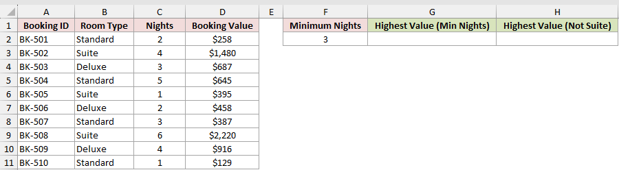
I want the highest value for stays meeting the minimum nights, then the highest value for rooms other than Suites.
Here is the formula:
=MAXIFS(D2:D11,C2:C11,">="&F2)
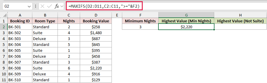
And here is the formula that excludes Suites:
=MAXIFS(D2:D11,B2:B11,"<>Suite")
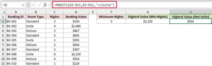
The first criterion joins >= to F2, where the minimum is three nights. It returns $2,220.
The second criterion uses <>, which means not equal to. After excluding Suites, the highest booking value is $916.
Pro Tip: Put comparison operators inside quotation marks. When the threshold is stored in a cell, join the operator and cell reference with an ampersand.
Example 4: MAXIFS for a Date Range
Here’s how to limit the calculation to one month.
Below is the dataset of museum attendance, with dates and daily visitor counts spanning February through April.
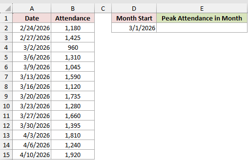
I want the peak attendance during the month beginning on the date in D2.
Here is the formula:
=MAXIFS(B2:B15,A2:A15,">="&D2,A2:A15,"<"&EDATE(D2,1))
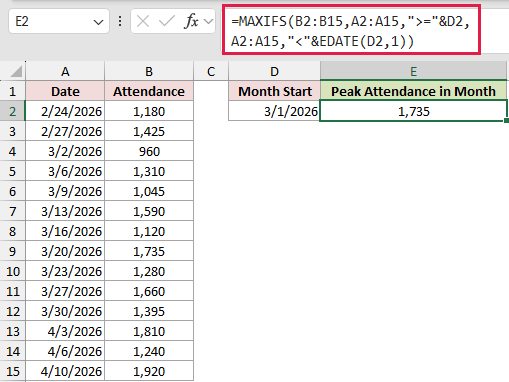
The first date criterion includes March 1 and later. The second excludes April 1 and later by using EDATE to set the upper boundary.
The peak attendance for March is 1,735.
Example 5: MAXIFS with Wildcards
Now let’s match partial text in client names.
Below is the dataset of clients and invoice amounts, including several names that start with Bay or end with LLC.
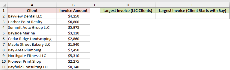
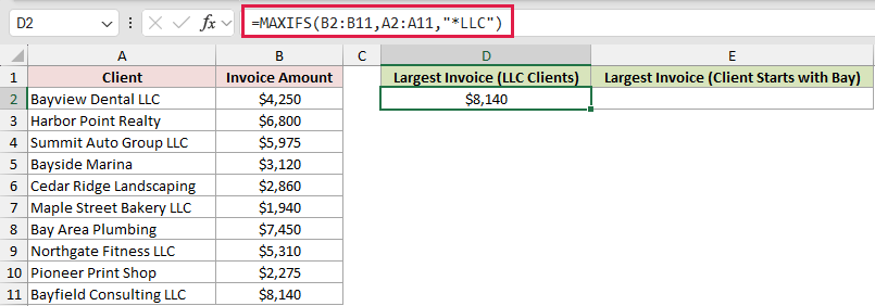
I want the largest invoice for LLC clients, then the largest invoice for client names beginning with Bay.
Here is the formula:
=MAXIFS(B2:B11,A2:A11,"*LLC")
And here is the formula for names beginning with Bay:
=MAXIFS(B2:B11,A2:A11,"Bay*")
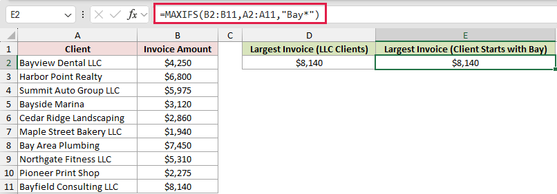
The asterisk matches any number of characters. Placing it before LLC finds names ending with LLC, while placing it after Bay finds names beginning with Bay.
Both formulas return $8,140 because Bayfield Consulting LLC satisfies both patterns and has the largest qualifying invoice.
Pro Tip: Use a question mark to match one character. Add a tilde before an asterisk or question mark when you need to match the symbol itself.
Example 6: Latest Date and No-Match Handling
This example shows a common date-formatting trap.
Below is the dataset of project tasks and due dates, plus two project names to check.
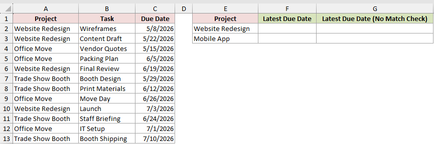
I want each project’s latest due date, with a friendly message when the project has no matching tasks.
Here is the formula:
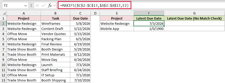
=MAXIFS($C$2:$C$13,$A$2:$A$13,E2)
And here is the formula with the no-match check:
=IF(COUNTIF($A$2:$A$13,E2)=0,"No tasks found",MAXIFS($C$2:$C$13,$A$2:$A$13,E2))
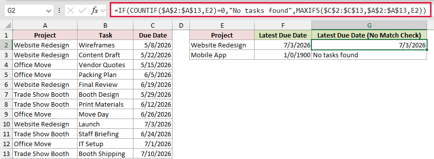
For Website Redesign, both formulas return July 3, 2026, the latest matching due date.
Copy both formulas down to row 3 for the Mobile App project. It has no match, so the plain MAXIFS result is zero.
Because that zero is date-formatted, Excel displays it as 1/0/1900. The guarded formula instead returns No tasks found.
Pro Tip: MAXIFS returns zero when no rows match. Check for matches first when zero could be mistaken for a valid number or date.
Example 7: MAXIFS per Group with a Spill
Let’s finish with a dynamic array example.
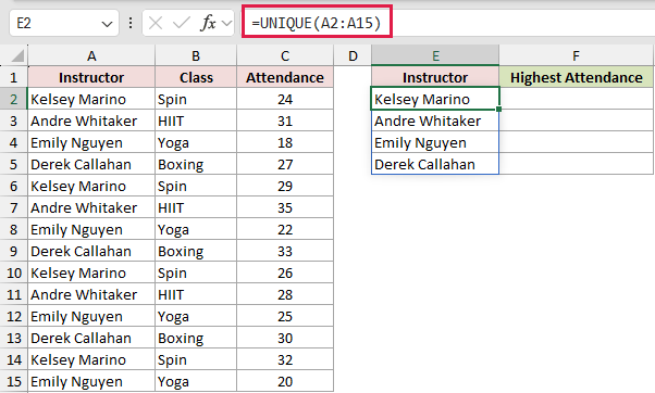
Below is the dataset of fitness classes, with instructor names, class types, and attendance figures.
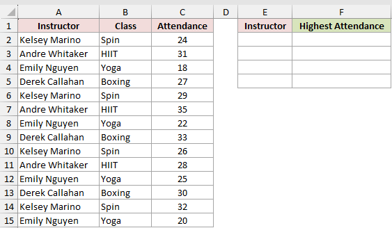
I want one spilled list of instructors and each instructor’s highest attendance.
Here is the formula:
=UNIQUE(A2:A15)
And here is the MAXIFS formula:
=MAXIFS(C2:C15,A2:A15,E2:E5)
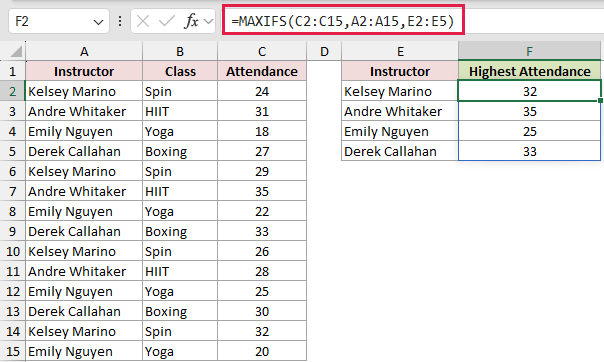
UNIQUE spills four instructor names into E2:E5. MAXIFS evaluates that entire range and spills the matching maximums into F2:F5.
The results are 32 for Kelsey Marino, 35 for Andre Whitaker, 25 for Emily Nguyen, and 33 for Derek Callahan.
In Excel 365, =GROUPBY(A2:A15,C2:C15,MAX) can return the names and maximums in one spilled table. The MAXIFS method still works and is useful in earlier versions.
Tips & Common Mistakes
- Keep
max_rangeand every criteria range the same size and shape. Mismatched ranges return a#VALUE!error. - MAXIFS is not case-sensitive when it checks text criteria.
- Multiple criteria pairs use AND logic. For OR logic, calculate each alternative separately and take the larger result.
- A no-match result is zero, not an error. Add a separate match check when zero would be misleading.
- MAXIFS is available in Excel 2019, Excel 2021, Excel 2024, and Excel 365.
- In older versions, you can use MAX with a conditional array formula entered with Ctrl+Shift+Enter.
MAXIFS finds the largest value that meets your conditions. Keep the ranges the same size, and remember that no qualifying rows return zero.
Related Excel Functions / Articles:
