
If you want to turn a range into one continuous column, the TOCOL function gives you a short formula for the job.
In this article, I’ll show you how to flatten ranges, skip blanks, change the reading order, reshape tables, and combine lists.
TOCOL is a dynamic array function. It spills its results into the cells below.
TOCOL Function Syntax in Excel
The TOCOL function converts an array or range into a single column.
=TOCOL(array, [ignore], [scan_by_column])
- array (required) is the range or array you want to return as one column.
- ignore (optional) controls which values TOCOL skips. Use 0 to keep everything, 1 to skip blanks, 2 to skip errors, or 3 to skip both.
- scan_by_column (optional) controls the reading order. FALSE or an omitted value scans each row from left to right. TRUE scans each column from top to bottom.
When to Use TOCOL Function
- Turn a table or grid into one continuous list, including TEXTSPLIT output when splitting text into rows.
- Remove blank cells or errors while flattening a range.
- Switch between row-by-row and column-by-column reading order.
- Reshape a cross-tab into a flat table for analysis.
- Build one sorted, distinct list from several columns, or every possible pairing from two lists.
Example 1: Flatten a Grid Into One Column
Let’s start with a weekly shift roster spread across five weekday columns.
Below is the dataset. Rows 2 through 5 contain four weeks of assignments, with weekdays in columns B through F.
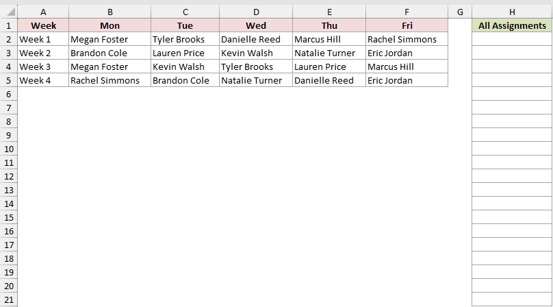
We want to turn all 20 assignments into one list in column H.
Here is the formula:
=TOCOL(B2:F5)
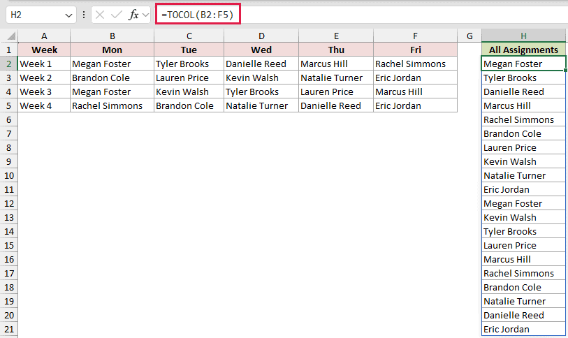
TOCOL reads the range from left to right across each row. It starts with the five Week 1 assignments, then moves to Week 2.
The formula in H2 spills through H21, so you enter it only once.
Pro Tip: Keep the cells below H2 empty. Any content in the intended spill range causes a #SPILL! error.
Example 2: Ignore Blank Cells With TOCOL
Here’s a volunteer schedule with several open time slots.
Below is the dataset. Columns B through E contain 20 station slots, including seven blank cells where nobody has signed up.
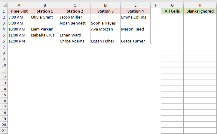
We first want to see how TOCOL handles the entire grid with its default settings.
Here is the formula:
=TOCOL(B2:E6)
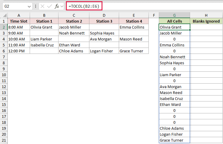
The formula returns 20 rows in column G. Each blank source cell appears as 0 because the default ignore value keeps blanks.
To return only the 13 volunteer names, use 1 for the ignore argument.
Here is the revised formula:
=TOCOL(B2:E6,1)
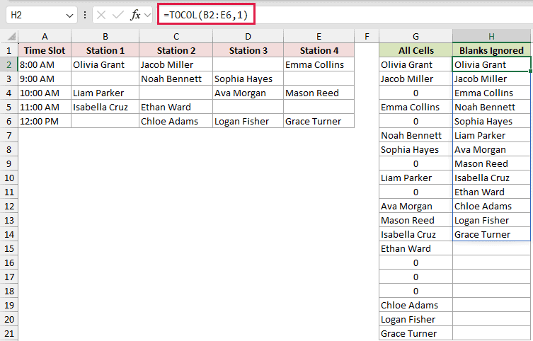
The second formula skips blank cells and spills the names from H2 through H14. Their original row-by-row order stays the same.
Pro Tip: Use 3 instead of 1 when the source may contain both blank cells and errors.
Example 3: Scan a Range by Column
Now let’s compare TOCOL’s two reading orders with monthly store sales.
Below is the dataset. Rows 2 through 5 list four stores, while columns B through D contain January, February, and March sales.
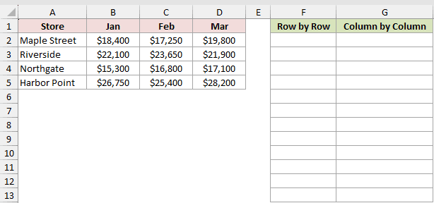
Let’s list the sales store by store, keeping each store’s three months together.
Here is the default row-scanning formula:
=TOCOL(B2:D5)
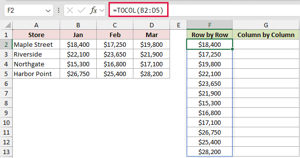
Column F starts with Maple Street’s $18,400, $17,250, and $19,800. It then moves to the three Riverside values.
To group every January value first, set scan_by_column to TRUE.
Here is the column-scanning formula:
=TOCOL(B2:D5,,TRUE)
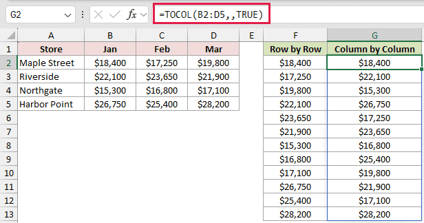
Column G starts with $18,400, $22,100, $15,300, and $26,750. Those are the January figures for all four stores.
The empty second argument keeps the default ignore setting. TRUE changes only the direction in which TOCOL reads the range.
Example 4: Unpivot a Cross-Tab With TOCOL
Let’s turn a department budget grid into a three-column table.
Below is the dataset. Department names run down column A, quarter names run across row 1, and budget values fill B2:E5.
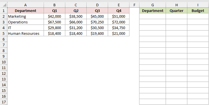
We want columns G through I to show one department, quarter, and budget combination per row.
Here is the department formula:
=TOCOL(IF(B2:E5<>"",A2:A5))
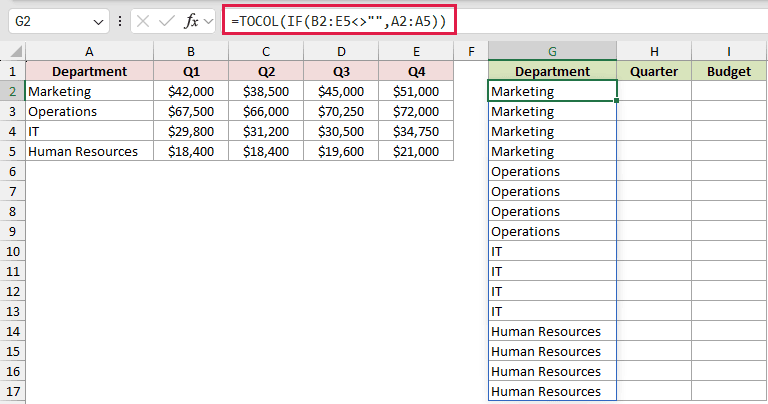
The IF function repeats each department name across the matching budget row. TOCOL then stacks those names in column G.
Here is the quarter formula:
=TOCOL(IF(B2:E5<>"",B1:E1))
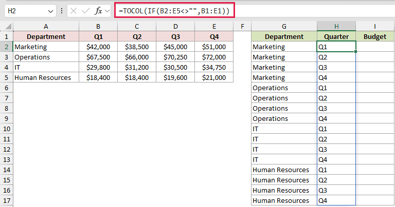
This IF formula repeats the quarter headers for every department. TOCOL places the resulting quarter labels in column H.
Here is the budget formula:
=TOCOL(B2:E5)
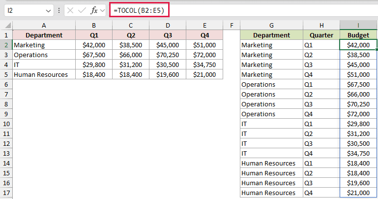
The third formula stacks the budget values in column I. Together, the three spills produce 16 records, starting with Marketing, Q1, and $42,000.
Power Query’s Unpivot Columns command is a better fit for large tables that need regular refreshes. TOCOL keeps this smaller result live on the worksheet.
Pro Tip: Keep all three spill areas clear. A blocked cell can stop one column from spilling and leave the flat table incomplete.
Example 5: Create a Sorted Distinct List
Here’s a useful way to combine TOCOL with two other dynamic array functions.
Below is the dataset. Each employee can have up to three skills in columns B through D, and some skill cells are blank.
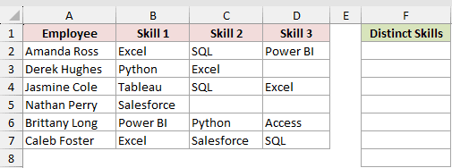
We want one alphabetized list containing each skill only once.
Here is the formula:
=SORT(UNIQUE(TOCOL(B2:D7,1)))
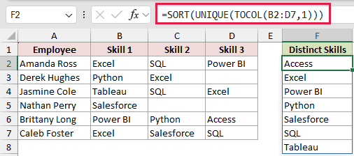
TOCOL first stacks the skill cells and ignores blanks. UNIQUE removes duplicates, and SORT arranges the remaining values alphabetically.
The result contains seven skills: Access, Excel, Power BI, Python, Salesforce, SQL, and Tableau.
Example 6: Merge Lists of Different Lengths
Finally, let’s combine two team lists when one column is shorter than the other.
Below is the dataset. Column A contains six East Team names, while column C contains four West Team names and two blank cells.
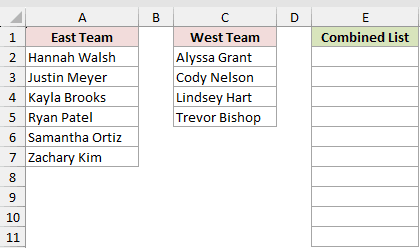
We want the six East names followed by the four West names in column E.
Here is the formula:
=TOCOL(HSTACK(A2:A7,C2:C7),3,TRUE)
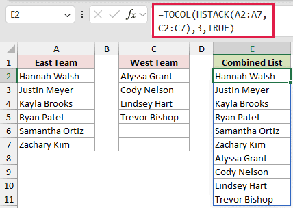
HSTACK places the two source lists side by side. TOCOL scans by column, so it reads the entire East list before the West list.
The ignore value 3 removes blank cells and any errors. The final spill contains exactly 10 names in E2:E11.
If both source lists have exact ranges, =VSTACK(A2:A7,C2:C5) is more direct. HSTACK with TOCOL is useful when lists have different or changing lengths and you want to reference the same row span for both.
Tips & Common Mistakes
- TOCOL is available in Microsoft 365 and Excel 2024. Older Excel versions do not support it.
- Blank cells appear as 0 unless you use 1 or 3 for the ignore argument.
- Use 2 to skip errors while keeping blanks. Use 3 to skip both errors and blanks.
- FALSE or an omitted scan_by_column argument reads across rows. TRUE reads down columns.
- A #SPILL! error means something is blocking the output range. Clear the cells where the results need to appear.
- TOCOL can return #VALUE! for array constants containing non-whole numbers, and #NUM! when the resulting array is too large.
Start with the default formula, then add the optional arguments only when your source contains blanks, errors, or needs a different reading order.
Related Excel Functions / Articles:
