
If you want to find cells where a formula has failed, the ISERROR function can flag every Excel error with TRUE.
In this article, I’ll show you how to spot, replace, count, and compare errors with practical ISERROR formulas.
In Excel 365, you can also feed ISERROR a range and the results will spill into the cells below.
ISERROR Function Syntax in Excel
The ISERROR function checks a value and returns TRUE when it is an error, or FALSE when it is not.
=ISERROR(value)
- value (required) is the value, cell reference, expression, or range you want to test for an error.
When to Use ISERROR Function
- Flag errors across a calculated column so you can find rows that need attention.
- Replace an error with a message or another value when ISERROR is combined with IF.
- Check whether a lookup failed before displaying its result.
- Count errors in imported data or exclude them from a calculation.
- Test for every error type instead of checking only for #N/A.
Example 1: Flag Errors with a Spilled Formula
Let’s start by checking a payroll calculation for errors.
Below is the dataset. Columns B and C contain hours and hourly rates, while column D calculates gross pay with =B2*C2 copied down.
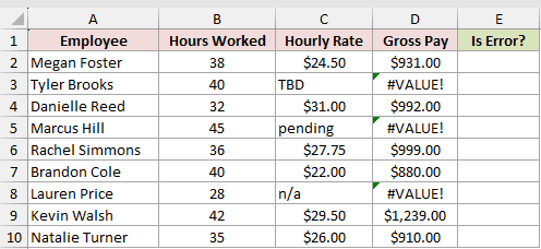
We want one ISERROR formula to flag every failed gross pay calculation in column D.
Here is the formula:
=ISERROR(D2:D10)
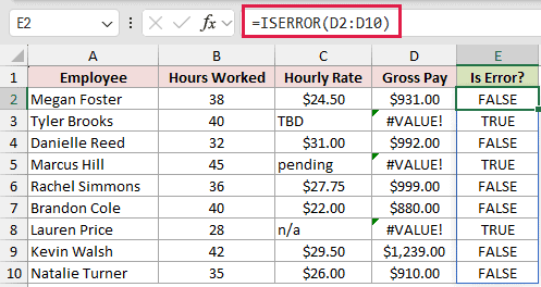
The formula checks all nine gross pay cells and spills TRUE or FALSE into E2:E10.
Rows 3, 5, and 8 return TRUE because their hourly rates contain text. The other rows return FALSE and calculate gross pay normally.
For example, Megan Foster’s gross pay is $931.00, while Danielle Reed’s is $992.00.
Pro Tip: Keep E2:E10 empty before entering the formula. A blocked spill range causes a #SPILL! error.
Example 2: Replace Division Errors with a Message
Here’s another practical scenario using advertising data.
Below is the dataset. Column B contains ad spend, column C contains clicks, and column D will calculate cost per click.

We want to show “No clicks” when division by zero would otherwise return an error.
Here is the formula:
=IF(ISERROR(B2:B9/C2:C9),"No clicks",B2:B9/C2:C9)
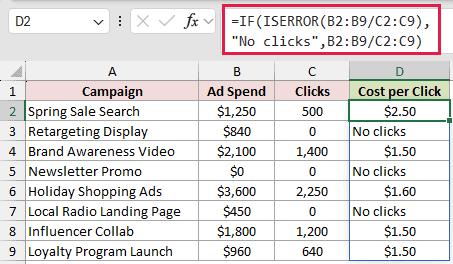
ISERROR tests each spend divided by clicks calculation. IF returns “No clicks” when that test is TRUE and returns the calculated cost when it is FALSE.
The valid costs per click are $2.50, $1.50, $1.60, $1.50, and $1.50. The three campaigns with zero clicks display the message.
In Excel 2007 or later, the IFERROR function does the same job with a shorter formula: =IFERROR(B2:B9/C2:C9,"No clicks").
The IF and ISERROR pattern still works in Excel 2003.
Example 3: Catch a Failed VLOOKUP with ISERROR
Now let’s check a volunteer list against a shift roster.
Below is the dataset. Column A lists volunteers, columns D and E contain the roster, and column B will return each assigned shift.
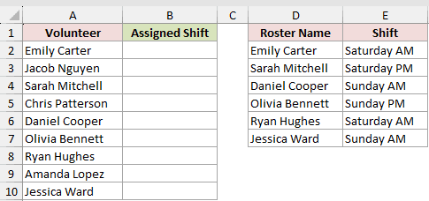
We want to return the matching shift or show “Not on roster” when VLOOKUP cannot find the volunteer.
Here is the formula:
=IF(ISERROR(VLOOKUP(A2:A10,$D$2:$E$7,2,FALSE)),"Not on roster",VLOOKUP(A2:A10,$D$2:$E$7,2,FALSE))
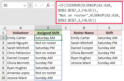
VLOOKUP searches the roster and returns a shift when it finds a match. ISERROR catches failed lookups, and IF replaces those errors with the message.
Jacob Nguyen, Chris Patterson, and Amanda Lopez are not on the roster. The other volunteers receive their Saturday or Sunday shifts.
In Excel 2021 and Microsoft 365, =XLOOKUP(A2:A10,D2:D7,E2:E7,"Not on roster") handles missing matches directly. IFNA with VLOOKUP is another option when you only want to catch #N/A.
Example 4: Count Errors and Sum Valid Values
Let’s step it up with imported invoice amounts.
Below is the dataset. Column B contains imported text, and column C uses =VALUE(B2) copied down to convert valid amounts into numbers.
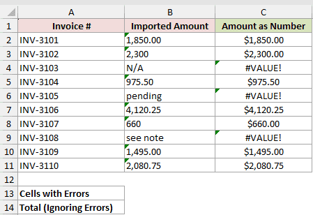
We first want to count the cells where the conversion in column C returned an error.
Here is the error-count formula:
=SUMPRODUCT(--ISERROR(C2:C11))
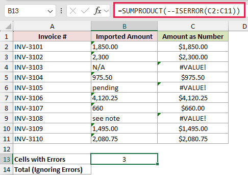
ISERROR creates TRUE and FALSE results. The double unary changes them to 1 and 0, then SUMPRODUCT adds the values and returns 3.
Next, we want to total the valid amounts while treating each error as zero.
Here is the total formula:
=SUM(IF(ISERROR(C2:C11),0,C2:C11))
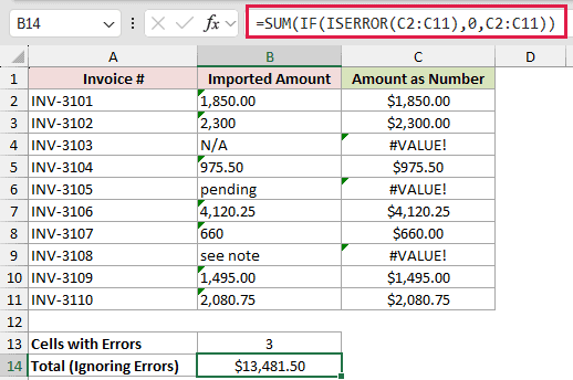
IF substitutes zero for each error and keeps every valid number. SUM then returns $13,481.50.
The errors come from “N/A,” “pending,” and “see note” in the imported amount column.
Pro Tip: =SUM(IFERROR(C2:C11,0)) is a shorter alternative when you want every error treated as zero.
Example 5: Compare ISERROR, ISERR, and ISNA
Finally, let’s compare three error-checking functions side by side.
Below is the dataset. Column B contains five error results, one number, and plain text. Columns C through E will test those values.
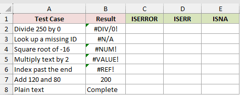
We want to see which values ISERROR, ISERR, and ISNA flag as errors.
Here is the ISERROR formula:
=ISERROR(B2:B8)
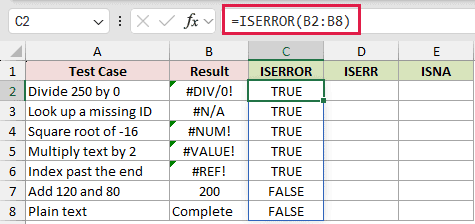
ISERROR returns TRUE for all five errors, including #N/A. It returns FALSE for the number and plain text.
Here is the ISERR formula:
=ISERR(B2:B8)
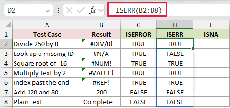
ISERR returns TRUE for the other four errors but FALSE for #N/A. It also returns FALSE for the number and text.
Here is the ISNA formula:
=ISNA(B2:B8)
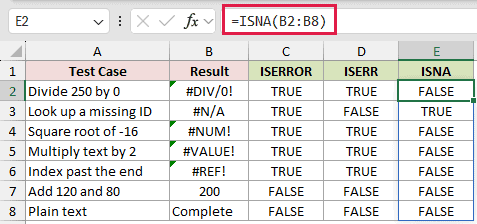
ISNA is the narrowest of the three checks. It returns TRUE only for #N/A and FALSE for every other value.
Use ISERROR when every error type matters, ISERR when #N/A should be excluded, and ISNA when you only need to identify #N/A.
Tips & Common Mistakes
- ISERROR catches #N/A, #VALUE!, #REF!, #DIV/0!, #NUM!, #NAME?, #NULL!, and newer errors such as #SPILL! and #CALC!.
- ISERROR does not convert text into numbers. For example,
=ISERROR("19")returns FALSE because the text value is not an error. - In Excel 365, a range-based ISERROR formula spills automatically. Make sure the output range is empty before entering it.
- Adding
@before ISERROR forces implicit intersection and reduces a range calculation to one result. Remove it when you want the full spilled array. - In older Excel versions, use a formula on each row and copy it down. Array calculations may require Ctrl + Shift + Enter.
- You can use
=ISERROR(D2)as a conditional formatting rule to highlight rows where a calculation failed.
ISERROR gives you a broad check for any Excel error. You can use that TRUE or FALSE result to flag problems or replace errors.
Use ISERR or ISNA instead when you need to treat #N/A differently from other errors.
Related Excel Functions / Articles:
