
COUNTIF counts matches in Excel, while VLOOKUP returns one value. Together, they can count orders by customer name when the order log stores only customer IDs.
You may also want to check for missing products or duplicate entries before trusting a lookup result.
I’ll cover counting by a looked-up ID and checking whether values exist. I’ll also show you how to flag duplicates and find second or Nth matches using a helper column.
Count How Many Times a Looked-Up Value Appears
You know the customer’s name, but you can’t count that name in an order log that only stores customer IDs.
I use VLOOKUP to find the customer’s ID first, then COUNTIF to count their orders.
Below I have 12 orders on the Count Orders sheet in A1:C13, with Order ID, Customer ID, and Amount headers. The orders store customer IDs only.
The name-to-ID list in E1:F6 has Customer Name and Customer ID headers. I’ve typed Harbor Bakery in H2, beneath the Customer Name header in H1.
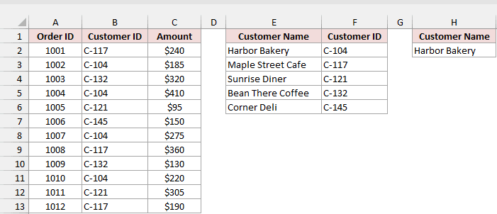
To count its orders, you can enter this formula in I2, beneath the Orders header in I1.
=COUNTIF(B2:B13,VLOOKUP(H2,E2:F6,2,FALSE))
The formula returns 4 orders for Harbor Bakery.
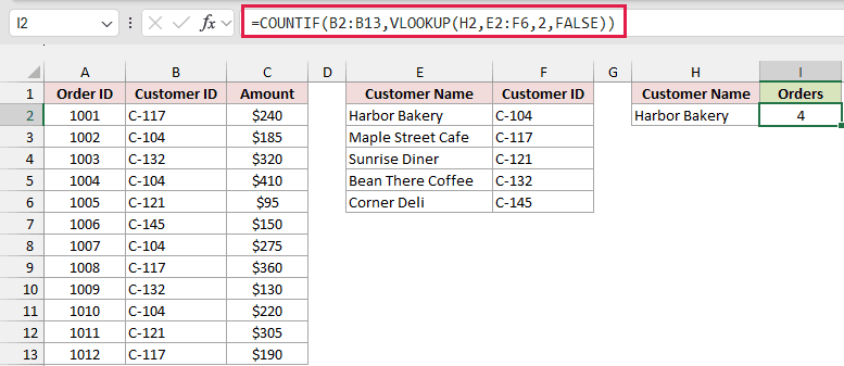
How does this formula work?
I first use VLOOKUP(H2,E2:F6,2,FALSE) to find Harbor Bakery in E2:E6. It returns C-104 from the second column. With FALSE, I ask for an exact match.
Then I use COUNTIF(B2:B13,"C-104") to count that ID in the order log.
The dataset has four matching orders, numbered 1002, 1004, 1007, and 1010, so the formula returns 4.
If you type Maple Street Cafe in H2, the formula returns 3 instead.
Note: If you mistype the name in H2 or enter one that isn’t in the customer list, VLOOKUP returns #N/A. COUNTIF doesn’t pass that error on. You get 0, which looks like the customer has no orders. You can check the name first with =IF(COUNTIF(E2:E6,H2)=0,"Customer not found",COUNTIF(B2:B13,VLOOKUP(H2,E2:F6,2,FALSE))). You get “Customer not found” for an unknown name, while Harbor Bakery still gives you 4.
Check If a Value Exists Before Running VLOOKUP
You can also use COUNTIF before a lookup to check whether the value exists in your list.
I’ll use that check to fetch unit prices and show “Not in list” for products that are missing.
Below I have order lines in A1:C8 on the Missing Values sheet, with Order ID, Product, and Unit Price headers.
The Unit Price column has a green header and empty cells. The price list in E1:F9 has Product and Unit Price headers.
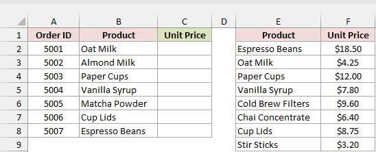
Almond Milk and Matcha Powder aren’t in the price list, so a plain VLOOKUP returns #N/A for both.
In Excel 365 or Excel 2021, you can enter this formula in C2.
=IF(COUNTIF(E2:E9,B2:B8)>0,VLOOKUP(B2:B8,E2:F9,2,FALSE),"Not in list")
You enter it once, and it fills C2:C8 automatically. That’s called spilling, so you don’t need to copy it down.
The formula returns $4.25, “Not in list”, $12.00, $7.80, “Not in list”, $8.75, and $18.50 in C2:C8, in that order.
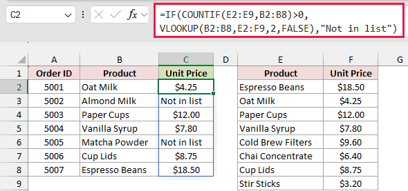
How does this formula work?
I use COUNTIF(E2:E9,B2:B8) to count how often each ordered product appears in the price list. It returns either 1 or 0 for each product here.
For a count above 0, I use VLOOKUP to fetch the price. Otherwise, the formula returns “Not in list”.
If you have an older Excel version, you can enter this formula in C2 and copy it down to C8.
=IF(COUNTIF($E$2:$E$9,B2)>0,VLOOKUP(B2,$E$2:$F$9,2,FALSE),"Not in list")
I prefer this check to wrapping VLOOKUP in IFERROR, a function that replaces any error with your chosen message. You can accidentally hide a formula mistake with IFERROR.
For example, you could ask VLOOKUP for column 3 in this two-column price list.
=IFERROR(VLOOKUP(B2,$E$2:$F$9,3,FALSE),"Not in list")
IFERROR returns “Not in list” for Oat Milk even though it’s there. With the COUNTIF version and that same wrong column number, you’d see #REF! instead.
You can then fix the column number rather than looking for a product that isn’t missing.
Flag Duplicate Lookup Values With COUNTIF
You might find the product in your list and still get a price you shouldn’t trust.
When you have two prices for the same product, I use COUNTIF to flag the duplicate before accepting VLOOKUP’s result.
Below I have a price list in A1:B9 on the Duplicate Values sheet, with Product and Unit Price headers.
The three products to look up in D2:D4 are Oat Milk, Paper Cups, and Cup Lids, beneath the Product header.
Oat Milk appears in rows 3 and 6, priced at $4.25 and $4.60. This can happen when someone adds a price without deleting the old one.
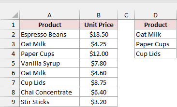
First, you can enter a plain VLOOKUP in E2, beneath the VLOOKUP Result header. In Excel 365 or Excel 2021, it spills down automatically.
=VLOOKUP(D2:D4,A2:B9,2,FALSE)
VLOOKUP returns $4.25 for Oat Milk, $12.00 for Paper Cups, and $8.75 for Cup Lids.
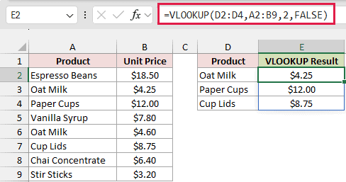
VLOOKUP returns $4.25 because it stops at the first match. It gives no warning about the second Oat Milk price of $4.60.
To flag that problem, you can enter this checked version in F2, beneath the Checked Result header. It also spills down automatically.
=IF(COUNTIF(A2:A9,D2:D4)>1,"Duplicate entry",VLOOKUP(D2:D4,A2:B9,2,FALSE))
The checked formula returns “Duplicate entry” for Oat Milk, followed by $12.00 for Paper Cups and $8.75 for Cup Lids.
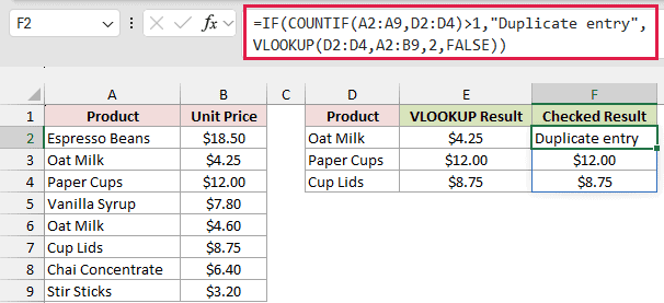
How does this formula work?
I use COUNTIF to count each product in A2:A9. For Oat Milk, it returns 2, which is more than 1, so the formula returns “Duplicate entry”.
For Paper Cups and Cup Lids, COUNTIF returns 1, so VLOOKUP returns their prices.
In older Excel versions, you can enter this formula in F2 and copy it down to F4.
=IF(COUNTIF($A$2:$A$9,D2)>1,"Duplicate entry",VLOOKUP(D2,$A$2:$B$9,2,FALSE))
Note: You can check for missing products and duplicates together with =IF(COUNTIF($A$2:$A$9,D2)=0,"Not in list",IF(COUNTIF($A$2:$A$9,D2)>1,"Duplicate entry",VLOOKUP(D2,$A$2:$B$9,2,FALSE))). If you type Almond Milk in D2, you get “Not in list”. Oat Milk still gives “Duplicate entry”, and Paper Cups gives $12.00.
Get the Second or Nth Match With a COUNTIF Helper Column
You don’t always want the first match. You may need the amount of a customer’s second order, or another occurrence further down the list.
I’ll give each order a unique label using COUNTIF, then use VLOOKUP to find the occurrence you ask for.
Below I have 10 orders in A1:C11, with Order ID, Customer, and Amount headers.
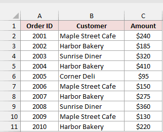
Harbor Bakery has four orders. A plain VLOOKUP on that name always returns the first amount, $185.
I’ll fetch the second order’s amount instead.
Step 1. Add a helper column
You need a new column for the labels you’ll look up. This extra column is called a helper column.
Right-click the column A header and choose Insert. The original data moves to B:D, with Customer now in column C.
Type Helper Key in A1. You can enter this formula in A2 and copy it down to A11.
=C2&"-"&COUNTIF($C$2:C2,C2)
You copy this one down rather than spilling it because the growing range is what does the counting.
The formula returns labels such as Harbor Bakery-1 and Harbor Bakery-2, with Harbor Bakery-4 on its fourth order.
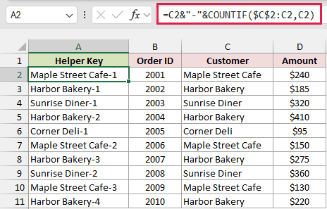
How does this formula work?
I use $C$2:C2 to count from the first customer cell to the current row. The dollar signs lock the start, while the end moves.
In A5, COUNTIF checks $C$2:C5. Harbor Bakery appears twice in that range, so COUNTIF returns 2.
I use & to join the customer name, a hyphen, and that count. The formula returns Harbor Bakery-2 in A5.
You now have a unique label for each order, so you can ask VLOOKUP for a particular occurrence.
Step 2. Look up the order you want
You can set up a small input box in F1:H2, with Customer, Occurrence, and Amount as the headers.
Type Harbor Bakery in F2 and 2 in G2. You can then enter this formula in H2.
=VLOOKUP(F2&"-"&G2,A2:D11,4,FALSE)
The formula returns $410, the amount for Harbor Bakery’s second order, order 2004.
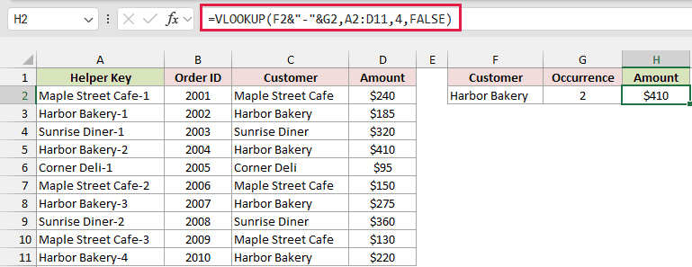
I use F2&"-"&G2 to build Harbor Bakery-2. VLOOKUP finds that label in the helper column and returns the value from the fourth column, Amount.
If you change G2 to 3, the formula returns $275. You can ask for any occurrence the customer has in the list.
To fetch the Order ID instead, change the column number from 4 to 2. For Harbor Bakery’s second order, the formula returns 2004.
If you ask for occurrence 5, the formula returns #N/A because Harbor Bakery only has four orders.
Note: You must keep the helper column first in your VLOOKUP table, A2:D11 here. VLOOKUP only searches the leftmost column.
Additional Notes About Using COUNTIF with VLOOKUP in Excel
You can avoid some confusing results by checking these details when you combine the functions.
- Both functions ignore capitalization. In the first example, the formula still returns 4 if you type “harbor bakery”.
- Use FALSE as VLOOKUP’s last argument for these examples. Approximate match on unsorted data can return the wrong row without an error.
- Keep lookup values and list entries the same data type. COUNTIF treats the number 104 and text “104” alike, so your existence check can pass while VLOOKUP returns #N/A.
- In the example file, the Nth Match sheet already has the helper column added, so the orders sit in B:D.
- In Excel 365 or Excel 2021, you can skip the helper column by using FILTER to collect matching amounts and INDEX to select the second one. Using those B:D columns,
=INDEX(FILTER(D2:D11,C2:C11="Harbor Bakery"),2)returns $410. - Use COUNTIFS when you need more than one condition.
Frequently Asked Questions
You may also be wondering which function does the counting or how to use these combinations with separate lists.
Can VLOOKUP count how many times a value appears?
No. VLOOKUP returns one value, the first match. You need COUNTIF to count matching entries, which is why I combine them.
Does COUNTIF with VLOOKUP work across two sheets?
Yes. You can point each range at its sheet. For example, you could count customer IDs on Orders and look up the name on Customers.
=COUNTIF(Orders!B2:B13,VLOOKUP(H2,Customers!A2:B6,2,FALSE))
You’d replace those illustrative sheet names and ranges with the ones in your workbook.
Should I use XLOOKUP instead of VLOOKUP?
In Excel 365 or Excel 2021, you can use XLOOKUP to fetch a value and supply a message through its built-in “if not found” argument.
This formula uses the Missing Values example from earlier, with Product in column B and the price list in E:F.
=XLOOKUP(B2,E2:E9,F2:F9,"Not in list")
You still need COUNTIF for the counting and duplicate checks. XLOOKUP handles the lookup part of the job.
Conclusion
I’d reach for COUNTIF(range,VLOOKUP(...)) when you know a name but need to count its ID in another list.
When you need to trust a fetched value, I like IF(COUNTIF(...)) for checking missing or duplicate entries before VLOOKUP picks a result.
I hope these examples help you choose a check, or use the COUNTIF helper column to find the second or Nth match.
Other Excel articles you may also like:
