
If you want to run the same calculation across every row of a table, the BYROW function can replace a set of copied formulas.
I’ll show you how to build both simple and more detailed row calculations with BYROW.
BYROW is a dynamic array function. It returns one result for each row and spills those results into the cells below.
BYROW Function Syntax in Excel
The BYROW function passes each row of an array to a LAMBDA and returns one result for that row.
=BYROW(array, lambda(row))
- array (required) is the range or array you want Excel to process one row at a time.
- lambda (required) is a LAMBDA that accepts one row and returns one value. The parameter name can be any valid Excel name.
When to Use BYROW Function
- Calculate a total, average, maximum, or minimum for every row with one formula.
- Count values in each row that meet a condition.
- Ignore selected values, such as zeros, before calculating a row result.
- Combine text from several columns into one value per row.
- Create a row-based condition for FILTER or another dynamic array function.
Example 1: Calculate Row Totals With BYROW
Let’s start by totaling monthly sales for each sales rep.
Below is the dataset. Column A lists the reps, and columns B through E contain their monthly sales.
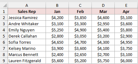
We want one BYROW formula in F2 to calculate and spill a total for every rep.
Here is the formula:
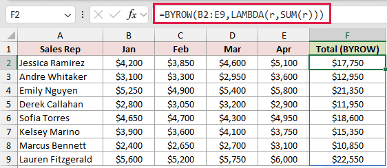
=BYROW(B2:E9,LAMBDA(r,SUM(r)))
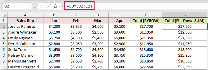
To see why BYROW is easier to maintain, compare it with the manual SUM method. Enter this formula in G2 and copy it through G9:
=SUM(B2:E2)
BYROW passes each four-cell row to the LAMBDA. The name r represents the current row, and SUM returns its total.
The single formula sits in F2 and spills all eight totals through F9. There is nothing to copy down.
Jessica Ramirez’s total is $17,750, and Lauren Fitzgerald’s is $22,550.
The SUM method needs a separate formula in every row. You enter =SUM(B2:E2) in G2, then copy or drag it down through G9.
When you add rows, you must copy SUM into those new rows too.
If the data grows, point BYROW at the expanded range or a table. Every total updates from one formula, while the fill-down column needs new copies.
Pro Tip: Excel 365 also accepts the shorter form =BYROW(B2:E9,SUM). The full LAMBDA form is useful when the row calculation needs more than one step.
The later examples follow the same pattern: one formula for the table, with a different calculation inside the LAMBDA.
Example 2: Find Each Row’s Best Quarter
Quarterly reports often need both the highest value and the quarter when it occurred.
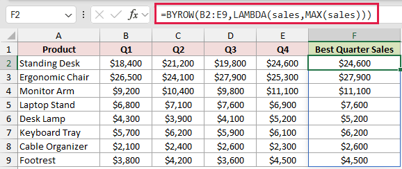
Below is the dataset. Column A lists products, and columns B through E contain their quarterly sales.
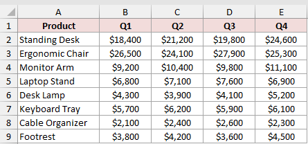
We want to return the highest sales figure and the matching quarter for every product.
First, here is the formula for the highest quarterly sales:
=BYROW(B2:E9,LAMBDA(sales,MAX(sales)))
To return the quarter name, use this second BYROW formula:
=BYROW(B2:E9,LAMBDA(sales,INDEX($B$1:$E$1,MATCH(MAX(sales),sales,0))))
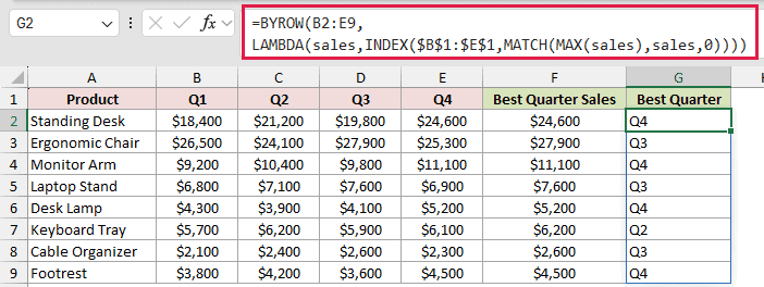
The first formula names the current row sales and uses MAX to return its largest value. Standing Desk returns $24,600, while Ergonomic Chair returns $27,900.
The second formula finds that maximum within the current row. MATCH returns its position, and INDEX uses that position to retrieve a heading from B1:E1.
The absolute reference $B$1:$E$1 keeps the quarter headings fixed while BYROW moves through the sales rows.
Pro Tip: If two quarters share the same maximum, MATCH returns the first one. Use a different approach when you need every tied quarter name.
Example 3: Count Values Below a Row Target
Performance reports often need a missed-target count for every carrier.
Below is the dataset. Column A lists freight carriers, and columns B through G show their monthly on-time percentages.
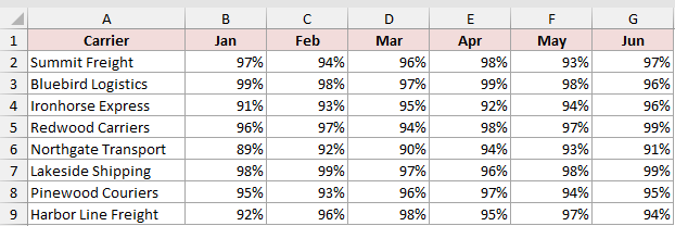
We want to count how many months each carrier fell below the 95% target.
Here is the formula:
=BYROW(B2:G9,LAMBDA(r,SUM(--(r<0.95))))
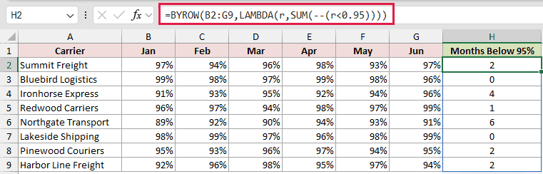
The test r<0.95 creates TRUE and FALSE results for the six values in each row. The double unary changes them to 1 and 0.
SUM then counts the 1s. Summit Freight missed the target twice, while Northgate Transport missed it in all six months.
A value of exactly 95% is not counted because the condition uses less than, not less than or equal to.
Pro Tip: COUNTIF expects a worksheet range and can be unreliable with the row array passed by BYROW. The SUM(--(condition)) pattern handles that array directly.
Example 4: Average Each Row While Ignoring Zeros
Closed days should not reduce a store’s average daily sales.
Below is the dataset. Column A lists stores, and columns B through H contain their daily sales.
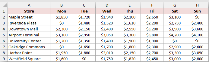
We want an average for each store that excludes every zero in its row.
Here is the formula:
=BYROW(B2:H9,LAMBDA(day,AVERAGE(FILTER(day,day>0))))
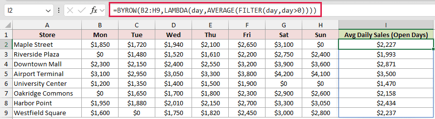
FILTER keeps only values greater than zero from the current day row. AVERAGE then calculates the result from those remaining values.
Maple Street averages $2,227 across six open days. University Center averages $1,470 across five open days, so its two closed days do not reduce the result.
Pro Tip: A row containing only zeros returns #CALC! because FILTER has no values to pass to AVERAGE. Add an error check if that can happen.
Example 5: Join Text Across Each Row
BYROW can process text as well as numbers.
Below is the dataset. Column A lists products, and columns B through D contain their optional tags.
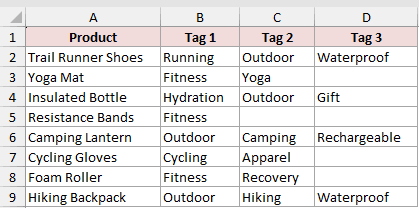
We want to join the available tags on each row and separate them with a slash.
Here is the formula:
=BYROW(B2:D9,LAMBDA(tags,TEXTJOIN(" / ",TRUE,tags)))
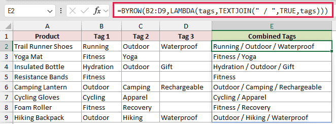
The LAMBDA names the current row tags and passes it to TEXTJOIN. The TRUE argument tells TEXTJOIN to ignore empty cells.
Trail Runner Shoes returns “Running / Outdoor / Waterproof”. Yoga Mat returns “Fitness / Yoga” without an extra separator for its blank third tag.
Example 6: Filter Rows by Their Total
Finally, let’s use BYROW to create the include condition for FILTER.
Below is the dataset. Column A lists customers, and columns B through D contain their January through March sales.
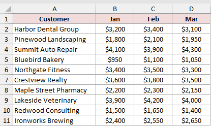
We want to keep only customers whose January through March sales total more than $10,000.
Here is the formula:
=FILTER(A2:D11,BYROW(B2:D11,LAMBDA(r,SUM(r)))>10000)
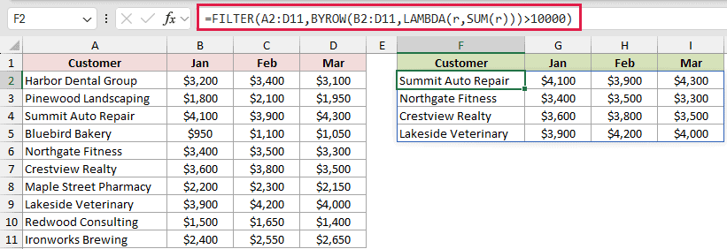
The inner BYROW formula calculates a three-month total for every customer. Comparing those totals with 10,000 creates the TRUE and FALSE values FILTER needs.
FILTER returns four matching rows in F2:I5. They are Summit Auto Repair, Northgate Fitness, Crestview Realty, and Lakeside Veterinary.
The condition uses greater than, so a customer totaling exactly $10,000 would not be included.
Tips & Common Mistakes
- BYROW is available in Excel for Microsoft 365 and Excel 2024. Earlier versions return #NAME? because they do not support the function.
- The LAMBDA must accept exactly one parameter and return one value for each row. An invalid LAMBDA can return #VALUE!, while a multi-value result can return #CALC!.
- Keep the spill range clear. A value in any required output cell causes #SPILL! and prevents BYROW from returning the row results.
- The LAMBDA parameter name is your choice. Short names such as
rwork well, but descriptive names such assales,day, ortagscan make longer formulas easier to follow. - Use BYCOL when you need one result per column. Use MAP when you need to apply a LAMBDA to individual values rather than complete rows.
- Do not add the
@operator before BYROW. It applies implicit intersection and can reduce a spilling calculation to one result.
Make sure the LAMBDA returns exactly one value for each row it receives.
Related Excel Functions / Articles:
