
If you want to turn numbers stored as text into real numbers, the VALUE function gives you a reliable formula-based method.
You’ll see how VALUE converts common imported text into numbers you can use in calculations.
In Excel 365, you can also feed VALUE a range and the results will spill into the cells below.
VALUE Function Syntax in Excel
The VALUE function converts recognized number, date, or time text into its numeric equivalent.
=VALUE(text)
- text (required) is the text string or cell reference you want to convert into a number.
When to Use VALUE Function
- Convert numbers imported from another system when Excel has stored them as text.
- Turn currency or percentage text into values that SUM and AVERAGE can calculate.
- Convert time or date text into Excel serial values for further calculations.
- Extract numeric parts from text codes and remove leading zeros.
- Handle columns where valid numbers are mixed with labels or other unwanted text.
Example 1: Convert Numbers Stored as Text With VALUE
Let’s start with a warehouse export where the shipped quantities arrived as text.
Below is the dataset. Column A lists order IDs, and column B contains the shipped quantities stored as text.
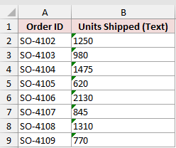
We want one VALUE formula to convert all eight quantities into numbers.
Here is the formula:
=VALUE(B2:B9)
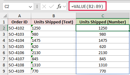
The formula reads the text values in B2:B9 and spills the converted numbers into C2:C9.
To see why VALUE is needed, here is what happens when SUM uses the original text column:
=SUM(B2:B9)
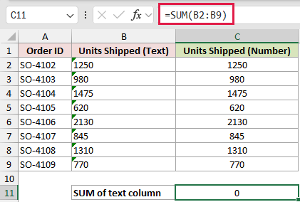
The result is 0 because SUM ignores numbers stored as text in worksheet cells.
Now compare that with SUM using the converted values:
=SUM(C2:C9)
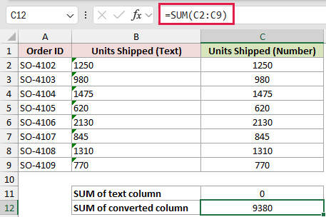
This time, SUM returns 9,380. The values in column C are real numbers, so Excel includes them in the calculation.
Pro Tip: If the spill range in C2:C9 is not empty, Excel returns #SPILL!. Clear those cells and enter the formula again.
Example 2: Use VALUE With Currency Text
Here’s another common import problem. The invoice totals include dollar signs and commas, but they are stored as text.
Below is the dataset. Column A lists vendors, and column B contains the imported invoice totals stored as text.
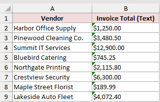
We want to convert every invoice total before calculating the amount payable.
Here is the conversion formula:
=VALUE(B2:B9)
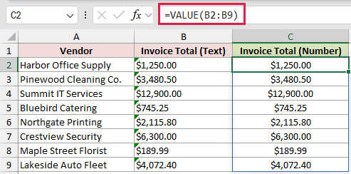
VALUE recognizes the dollar signs and thousands separators, then spills the numeric amounts into column C.
Here is the total formula:
=SUM(C2:C9)
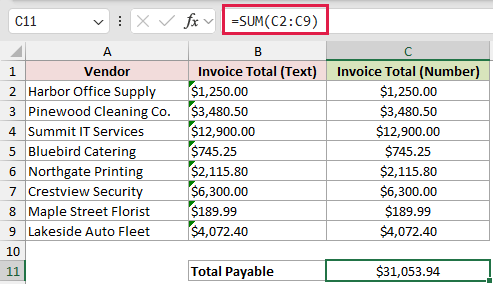
SUM now returns a total payable of $31,053.94.
VALUE follows your system’s number separators. If the imported text uses different separators, NUMBERVALUE is a better choice because you can specify them explicitly.
Pro Tip: A value such as 1.250,00 may fail or be misread on a system that expects commas for thousands and periods for decimals.
Example 3: Convert Percentage Text to Percentages
Percentage values copied from an email reporting tool often need the same cleanup.
Below is the dataset. Column A lists email campaigns, and column B contains open rates stored as text.
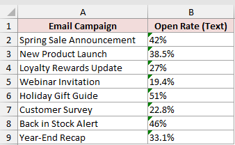
We want to convert all eight open rates and then calculate their average.
Here is the conversion formula:
=VALUE(B2:B9)
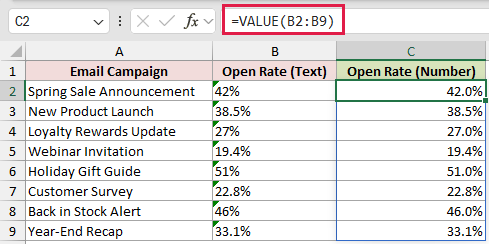
VALUE converts 42% into 0.42 and 38.5% into 0.385. Percentage formatting makes those decimal values display with percent signs.
Here is the average formula:
=AVERAGE(C2:C9)
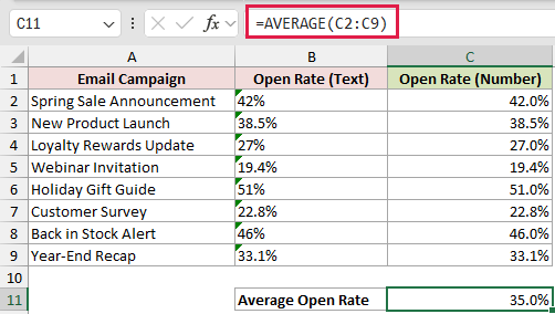
The underlying average is 34.975%. With the workbook’s one-decimal percentage format, Excel displays it as 35.0%.
Pro Tip: VALUE converts the data but does not choose its display. Apply Percentage format if Excel shows results such as 0.42 instead of 42%.
Example 4: Extract Numbers From Text Codes
Let’s combine VALUE with RIGHT to turn equipment tags into numeric meter numbers.
Below is the dataset. Column A contains the meter tags.
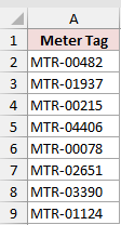
We want to take the last five characters from every tag and convert them into numbers.
Here is the formula:
=VALUE(RIGHT(A2:A9,5))
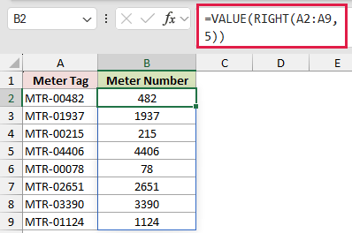
RIGHT extracts five text characters from each tag. VALUE converts those characters, so MTR-00482 becomes 482 and MTR-00078 becomes 78.
In Excel 365, =VALUE(TEXTAFTER(A2:A9,"-")) avoids counting characters. The RIGHT version remains useful in older Excel versions that do not include TEXTAFTER.
Pro Tip: VALUE removes leading zeros. Keep the extracted result as text if 00482 is an identifier that must retain all five digits.
Example 5: Convert Time Text to Hours Worked
Imported clock times create a different kind of calculation problem.
Below is the dataset. Column A lists employees, while columns B and C contain the clock-in and clock-out times stored as text.
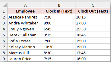
We want to convert both time columns and subtract each clock-in time from its matching clock-out time.
Here is the formula:
=VALUE(C2:C9)-VALUE(B2:B9)
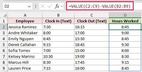
VALUE converts each time into Excel’s time serial number. Subtraction then returns the elapsed part of a day for every row.
The [h]:mm format displays those decimals as durations. Jessica’s 7:30 to 16:15 shift shows 8:45, while Derek’s shift shows 9:30.
TIMEVALUE is the purpose-built option for time text. The equivalent range formula is =TIMEVALUE(C2:C9)-TIMEVALUE(B2:B9), while VALUE also handles other recognized number formats.
Pro Tip: This subtraction assumes the clock-out time is later on the same day. An overnight shift needs an adjustment for the date change.
Example 6: Handle Invalid Text With IFERROR
Finally, let’s clean a sensor column containing numbers and status labels.
Below is the dataset. Column A lists sensors, while column B mixes reported readings with N/A, double hyphens, and Offline entries.
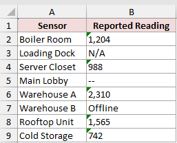
We want to compare plain VALUE with a version that leaves invalid rows blank.
Here is the plain VALUE formula:
=VALUE(B2:B9)
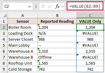
VALUE converts the valid readings, including 1,204 and 2,310. It returns #VALUE! in C3, C5, and C7 for the three unrecognized entries.
To show how IFERROR changes the outcome, here is the error-handling formula:
=IFERROR(VALUE(B2:B9),"")
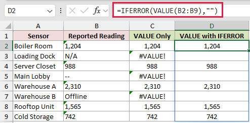
IFERROR keeps each successful conversion and replaces every error with an empty string. The affected cells look blank in column D.
Pro Tip: Blank output keeps reports tidy, but it can hide bad source data. Check the rejected entries before relying on the cleaned column.
Tips & Common Mistakes
- Excel often converts text automatically during arithmetic, but SUM, AVERAGE, and COUNT can ignore text values stored in cells.
- VALUE uses the separators and recognized formats from your system settings. Use NUMBERVALUE when the source text follows a different locale.
- Dates and times become Excel serial numbers. Apply a date, time, or duration format to display them properly.
- VALUE removes leading zeros because numbers do not retain them. Keep identifiers such as ZIP codes and account codes as text.
- In Excel 365, range-based VALUE formulas spill automatically. Clear blocked cells if Excel returns #SPILL!.
- In older Excel versions, enter VALUE for the first row and copy the formula down instead of using a range argument.
- VALUE returns #VALUE! when Excel cannot recognize the text. IFERROR can replace that error, but check whether the source needs correction.
Use VALUE when text-looking numbers need to work in calculations.
Related Excel Functions / Articles:
