
Excel’s ISFORMULA function returns TRUE when a referenced cell contains a formula and FALSE when it does not. It checks the cell’s contents, not the displayed result.
A typed number can match a calculated result and still return FALSE. A formula that displays an error or an empty string still returns TRUE.
The examples build from a basic formula check to practical audits for typed-over values and blank-looking cells.
ISFORMULA Function Syntax in Excel
The ISFORMULA function uses the following syntax:
=ISFORMULA(reference)
- reference: Required. The cell or range you want to test. It can also be a formula that returns a reference or a name referring to a cell.
When to Use ISFORMULA Function
- Audit a calculated column for values that someone typed over.
- Distinguish formula cells from regular inputs, even when their displayed values look identical.
- Count formulas and typed values within a defined range.
- Find formulas that appear blank or return an error.
- Build a review list containing rows with hardcoded values.
Example 1: Check Cells for Formulas
Let’s start with the function’s basic test.
Below is the dataset with Order ID, Guests, Price per Guest, Order Total, and an empty Is Formula? column.
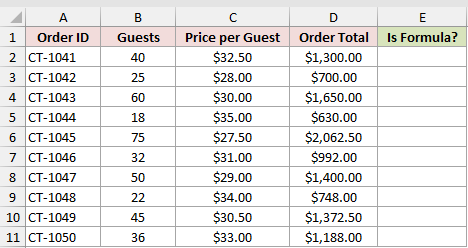
We want to check every cell in D2:D11 and return one TRUE or FALSE result in E2:E11.
Here is the formula:
=ISFORMULA(D2:D11)
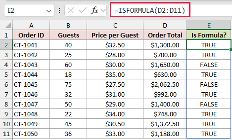
The formula checks each cell in D2:D11. For a manual view across the sheet, use the Show Formulas shortcut (<code>Ctrl+`</code>).
It spills TRUE for formulas and FALSE for typed values.
The first result in E2 is TRUE because D2 contains the Order Total formula =B2*C2.
CT-1045 returns FALSE because its Order Total is typed, even though $2,062.50 equals the result of multiplying 75 by $27.50.
Pro Tip: In Excel 2013 through 2019, use =ISFORMULA(D2) in each row and fill it down.
Example 2: Show Formula Text or Typed Values
Now let’s make the TRUE and FALSE test more descriptive.
Below is a trade show budget with Budget Item, Amount, and an empty How It’s Calculated column.
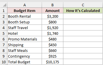
We want to display each formula from B2:B10 and label every typed amount as Typed value.
Here is the formula:
=IF(ISFORMULA(B2:B10),FORMULATEXT(B2:B10),"Typed value")
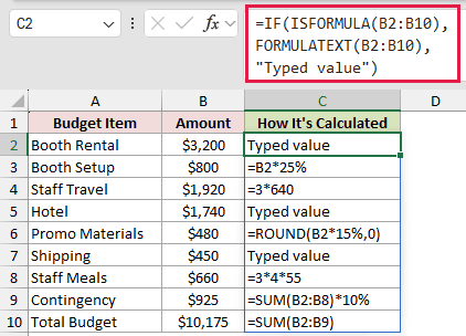
How this formula works:
ISFORMULA(B2:B10)tests each cell in the Amount column.IFpasses formula cells toFORMULATEXTand returnsTyped valuefor the other cells.FORMULATEXTreturns formula text such as=B2*25%and=3*640, exposing fixed numbers hidden inside formulas.
The first result in C2 is Typed value because B2 contains 3200 rather than a formula.
Example 3: Count Formula Cells and Typed Values
Here’s a quick way to summarize a mixed calculation column.
Below is the dataset with Month and Projected Revenue. The empty Formula Cells and Typed Values result cells sit below the monthly figures.
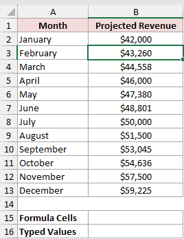
We want to count the formulas and typed values in B2:B13 separately.
Here is the formula:
=SUMPRODUCT(--ISFORMULA(B2:B13))
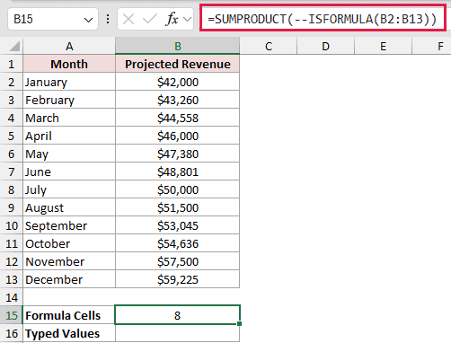
And here is the formula for Typed Values:
=SUMPRODUCT(--NOT(ISFORMULA(B2:B13)))
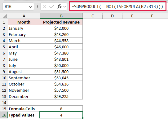
How these formulas work:
ISFORMULA(B2:B13)produces TRUE and FALSE values. The double unary converts them to 1 and 0, andSUMPRODUCTreturns 8.NOTreverses the test before the same conversion, so the second formula returns 4.- January is the expected starting input. The other typed values, April, July, and November, are the three overrides.
Pro Tip: In Excel 2021 and later, =SUM(--ISFORMULA(B2:B13)) is a shorter option. SUMPRODUCT still works in Excel 2013 through 2019.
Example 4: Find Hardcoded Values with ISFORMULA and FILTER
Next, let’s turn the audit into a focused review list.
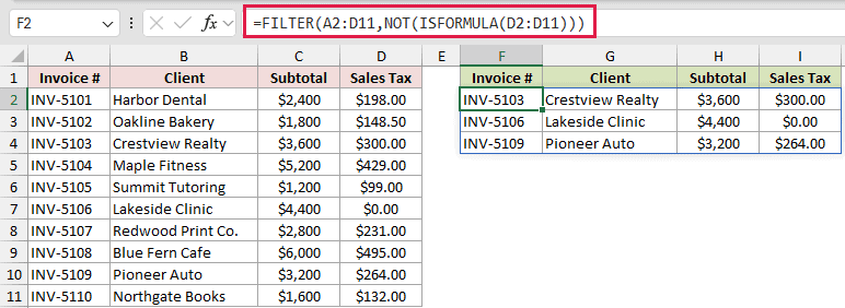
Below is the invoice dataset with Invoice #, Client, Subtotal, and Sales Tax. An empty output table appears on the right.
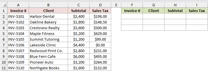
We want to return invoices where Sales Tax in D2:D11 is a typed value rather than a formula.
Here is the formula:
=FILTER(A2:D11,NOT(ISFORMULA(D2:D11)))
How this formula works:
ISFORMULA(D2:D11)returns TRUE for formula cells and FALSE for typed values.NOTreverses those results, making the typed Sales Tax entries TRUE forFILTER.FILTERreturns the matching rows from A2:D11 and spills INV-5103, INV-5106, and INV-5109 into F2:I4.
INV-5109 is included even though its typed Sales Tax of 264 matches what the column formula =C10*8.25% would return.
Pro Tip: FILTER works in Excel 2021, Excel 2024, and Microsoft 365. In Excel 2013 through 2019, use an ISFORMULA helper column with AutoFilter.
Example 5: Detect Deleted and Blank-Looking Formulas
This last example shows why visible blanks can be misleading.
Below is the dataset with Order ID, Order Amount, Loyalty Discount, and an empty Is Formula? column.
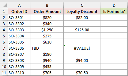
We want to tell blank-looking formula results from cells where the formula was deleted. We will also check whether an error cell still contains a formula.
Here is the formula:
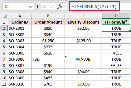
=ISFORMULA(C2:C11)
How this formula works:
ISFORMULA(C2:C11)checks whether each Loyalty Discount cell contains a formula, regardless of the displayed result.- SO-3302, SO-3304, and SO-3309 look blank because their formulas return
"". An ISBLANK check returns FALSE for those cells. - SO-3305 and SO-3307 return FALSE because their formulas were deleted. SO-3305 is missing a $61 discount.
- SO-3306 shows #VALUE! in C7, but D7 returns TRUE because C7 still contains a formula.
Tips & Common Mistakes
- ISFORMULA was introduced in Excel 2013.
- The argument must be a reference. A named constant returns #VALUE! because it does not refer to a cell.
- A formula stored as text returns FALSE because Excel treats it as text, not as a formula.
- For conditional formatting, use
=ISFORMULA(A1)to highlight formulas or=NOT(ISFORMULA(A1))to highlight hardcoded cells. - Leave the output range empty before entering a spilling formula. A blocked spill returns #SPILL! at the formula cell.
- Using NOT with ISFORMULA also identifies blank cells as not containing formulas. Keep counting ranges limited to the intended data.
I covered how ISFORMULA identifies formula cells and supports practical audits, even when displayed values are misleading.
I hope you found this article helpful.
Related Excel Functions / Articles:
Other Excel articles you may also like:
