IMCSCH Function in Excel (4 Easy Examples)

The IMCSCH function in Excel returns the hyperbolic cosecant of a complex number, which is the reciprocal of its hyperbolic sine.

The result is complex-number text, so changing the cell’s decimal format won’t shorten it. Even results that look like ordinary numbers remain text.

The examples cover extracting numeric parts from IMCSCH results and checking the reciprocal calculation when the output strings differ.

Table of Contents

IMCSCH Function Syntax in Excel

IMCSCH takes a single required argument:

=IMCSCH(inumber)

inumber (required): The complex number to evaluate, written as x+yi or x+yj. You can supply text, a cell reference, or a real number.

Use lowercase i or j for the imaginary suffix. COMPLEX can build the input when the real and imaginary parts occupy separate cells.

IMCSCH is available in Excel 2013 and later. Its input isn’t an angle, so don’t convert it with RADIANS.

When to Use IMCSCH Function

Calculate hyperbolic cosecants when your inputs contain real and imaginary parts.
Evaluate the reciprocal of a complex hyperbolic sine directly.

Example 1: Calculate and Read Complex Results

Let’s start with a column of complex numbers and separate the output into readable parts.

Below is the dataset. Columns A and B hold labels and complex inputs; columns C through E have headers for IMCSCH results and their numeric parts.

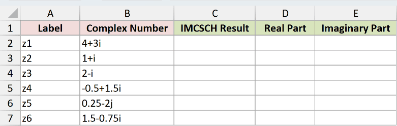
We want each input’s hyperbolic cosecant, followed by its rounded real and imaginary parts.

Enter this formula in C2, then copy it down to C7:

=IMCSCH(B2)

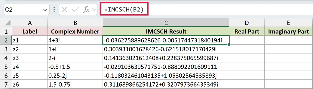
For 4+3i, cell C2 returns -0.036275889628626-0.0051744731840194i. The part before the imaginary term is real; the coefficient beside i is imaginary.

This output is text. To round it, extract the numeric parts first instead of applying ROUND to the complete complex string.

Enter the real-part formula in D2, then copy it down to D7:

=ROUND(IMREAL(C2),4)

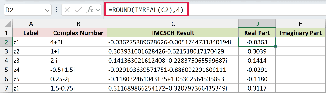
IMREAL extracts the real component, and ROUND shortens that number. Cell D2 displays -0.0363.

Enter the imaginary-part formula in E2, then copy it down to E7:

=ROUND(IMAGINARY(C2),4)

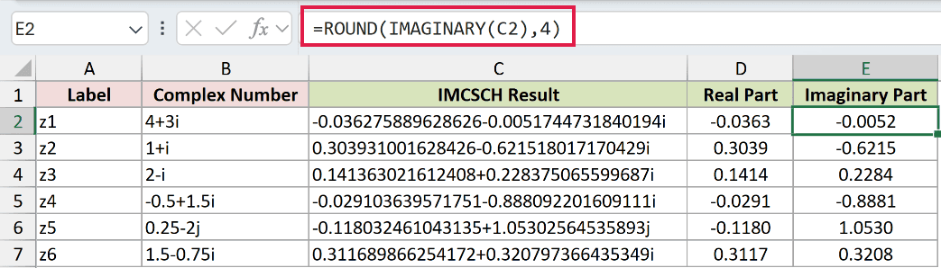
Cell E2 displays -0.0052. This is a usable number, without the imaginary suffix.

The 0.25-2j row keeps j in its complex result. Its extracted parts display -0.1180 and 1.0530, so the extraction also works with that suffix.

Pro Tip: Bare ranges return one #VALUE!. +range or range&"" spills in Excel 2021, 2024 and Microsoft 365. In Excel 2019 and earlier, fill down.

Example 2: Check the Reciprocal Without Comparing Text

Now let’s check the reciprocal relationship and see why a text equality test can mislead you.

Below is the dataset. Column A contains complex inputs; columns B through F provide spaces for hyperbolic sine, cosecant, reciprocal, numeric difference, and text comparisons.

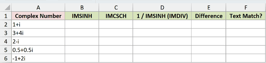
We want to compare IMCSCH with the reciprocal of IMSINH and measure any difference numerically.

First, calculate hyperbolic sine in B2 and copy down to B6:

=IMSINH(A2)

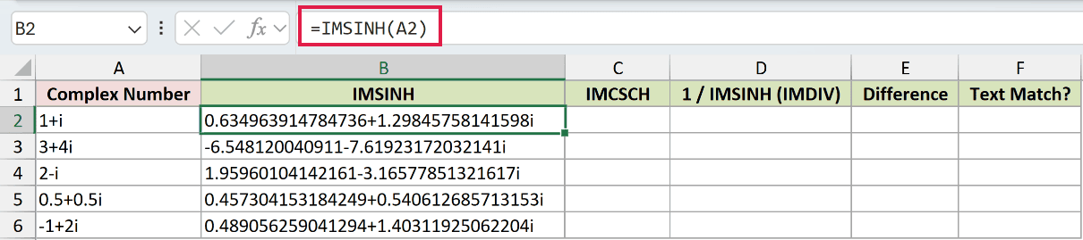
For 1+i, this returns 0.634963914784736+1.29845758141598i.

Calculate IMCSCH directly in C2 and copy down to C6:

=IMCSCH(A2)

Cell C2 returns 0.303931001628426-0.621518017170429i.

For the reciprocal comparison, enter this formula in D2 and copy down to D6:

=IMDIV(1,B2)

IMDIV divides by the complex hyperbolic sine in B2. The comparison result is 0.303931001628425-0.621518017170428i, with slightly different final digits.

Measure the numeric difference in E2, then copy down to E6:

=IMABS(IMSUB(C2,D2))

IMSUB subtracts the complex results. IMABS then returns the magnitude of that difference as a real number.

Cell E2 displays 1.4E-15. This tiny difference comes from rounding in the two calculation routes.

To demonstrate the misleading text comparison, enter this in F2 and copy down to F6:

=C2=D2

The Text Match? column is a comparison trap. It tests the output strings, so it isn’t a reliable check of numerical agreement.

1+i returns FALSE, with a Difference of 1.4E-15.
3+4i returns TRUE, with a Difference of 0.0E+00.
2-i returns FALSE, with a Difference of 1.0E-15.
0.5+0.5i returns TRUE, with a Difference of 0.0E+00.
-1+2i returns FALSE, with a Difference of 1.0E-15.

Use the Difference column to judge agreement at the precision your calculation needs. Don’t treat a FALSE text match as proof the reciprocal is wrong.

Example 3: Compare IMCSCH and CSCH

For real inputs, IMCSCH returns text and CSCH returns a number.

Below is the dataset. Column A holds real numbers, with an IMCSCH result column in B and a real-number CSCH comparison column in C.

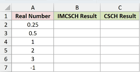
We want to compare complex-text output with CSCH’s ordinary numeric output on the same inputs.

Enter the IMCSCH formula in B2 and copy down to B7:

=IMCSCH(A2)

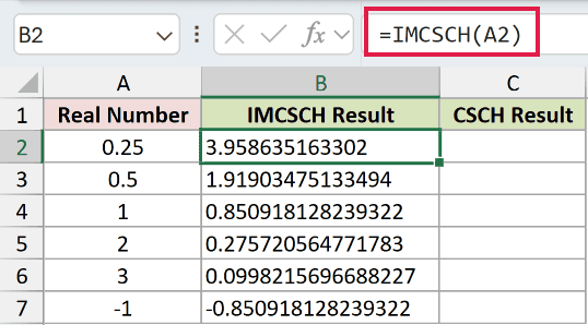
For the input 0.25, cell B2 returns 3.958635163302. It looks numeric, but IMCSCH still returns text.

For the real-number comparison, enter CSCH in C2 and copy down to C7:

=CSCH(A2)

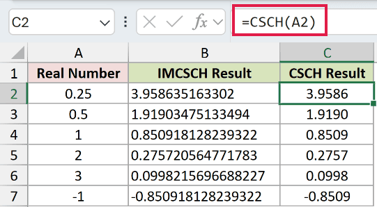
The CSCH comparison in C2 displays 3.9586 because its numeric result follows the cell’s decimal format.

For input 1, IMCSCH returns 0.850918128239322, while the CSCH comparison displays 0.8509.

Choose CSCH when your inputs are real and you need ordinary arithmetic afterward. Use IMCSCH when the calculation needs to handle complex inputs.

Example 4: Understand Errors and Extreme Inputs

Finally, let’s check the cases where the output can look surprising.

Below is the dataset. Column A labels each input check, column B contains the test values, and column C is reserved for IMCSCH results.

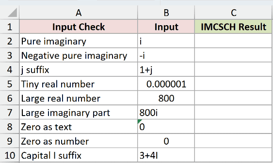
We want to distinguish valid edge-case results from deliberate input errors.

Enter this formula in C2, then copy it down to C10:

=IMCSCH(B2)

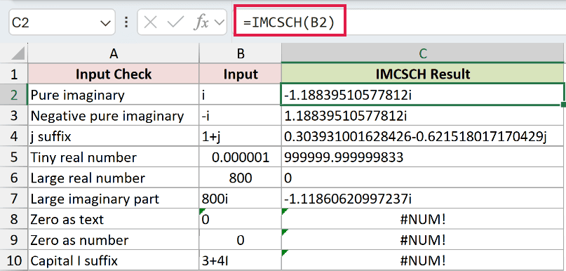
Each row demonstrates a different input check:

Pure imaginary, i: Cell C2 returns -1.18839510577812i. A purely imaginary input can produce a purely imaginary result.
Negative pure imaginary, -i: Cell C3 returns 1.18839510577812i. Reversing the input’s sign reverses the output’s sign, illustrating IMCSCH’s odd symmetry.
Lowercase j: Cell C4 returns 0.303931001628426-0.621518017170429j for 1+j. Excel preserves the suffix.
Tiny real input: The input 0.000001 returns 999999.999999833 in C5. Near zero, the reciprocal can become very large.
Large real input: The input 800 returns the text 0 in C6. The result is too small for Excel to represent, so it returns zero without raising an error.
Large imaginary input: The input 800i returns -1.11860620997237i in C7. A large imaginary part behaves differently from a large real part.
Zero stored as text: Cell C8 deliberately returns #NUM!. Hyperbolic cosecant is undefined at zero.
Zero stored as a number: Cell C9 also deliberately returns #NUM!. Changing the input’s storage type doesn’t remove the zero-input problem.
Capital suffix: The input 3+4I deliberately returns #NUM! in C10. Replace the uppercase suffix with lowercase i.

The error cells belong to the demonstration. Correct the underlying input when it’s a mistake in your own data.

Tips & Common Mistakes

Check empty inputs. A blank referenced cell is treated as zero, so IMCSCH returns #NUM!. An unfilled input isn’t skipped automatically.
Keep logical values out. A logical such as TRUE returns #VALUE!. Check the source cell if you expected complex-number text.
Extract numbers before ordinary calculations. Use IMREAL or IMAGINARY for individual components and IMABS for magnitude. Don’t directly sum a column of IMCSCH text results.
Keep hyperbolic and circular functions separate. IMCSCH uses hyperbolic sine. IMCSC uses ordinary complex sine; the names aren’t interchangeable.
Inspect the suffix before removing spaces. Capital I is invalid, but spaces within otherwise valid complex text were accepted in testing.

I’ve shown how to extract numeric parts from IMCSCH results and check reciprocal calculations. Use the numeric difference to judge agreement when the text outputs differ. <p class=”has-base-background-color has-background”><a href=”https://spreadsheetplanet.com/excel-functions/”><em>List of All Excel Functions</em></a></p> <!– /wp:paragraph –>

Other Excel articles you may also like: