IMSINH Function in Excel (4 Easy Examples)

The IMSINH function in Excel returns the hyperbolic sine of a complex number. Its result can contain both a real part and an imaginary part.

Excel stores that result as text, even when the imaginary part disappears. This matters when you want to format the answer or use it in ordinary calculations.

I’ll cover complex hyperbolic sine calculations alongside the real-number SINH comparison. We’ll also check answers through IMSIN and work through errors and overflow.

Table of Contents

IMSINH Function Syntax in Excel

IMSINH takes a single required argument:

=IMSINH(inumber)

inumber (required): The complex number whose hyperbolic sine you want. Supply complex text in x+yi or x+yj form, a real number, or a cell reference.

Use lowercase i or j for the imaginary suffix. When typing complex text directly into a formula, enclose it in double quotes.

You can also use COMPLEX to build the input from separate real and imaginary parts. IMSINH is available in Excel 2013 and later.

When to Use IMSINH Function

Calculate hyperbolic sines for complex values stored in worksheet cells.
Check how negating or conjugating an input changes its hyperbolic sine.
Verify a complex sine identity against a direct IMSINH result.

For inputs with no imaginary part, SINH is usually the better choice because it returns a number you can use directly.

Example 1: Calculate a Complex Hyperbolic Sine

Let’s start with complex inputs that make the sign changes easy to follow.

Below is the dataset. Column A labels each case, column B holds the complex inputs, and column C is reserved for their hyperbolic sines.

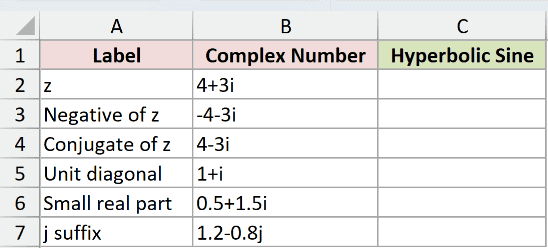
We want to calculate each input’s hyperbolic sine and compare the negative and conjugate cases.

Enter this formula in C2, then copy it down to C7:

=IMSINH(B2)

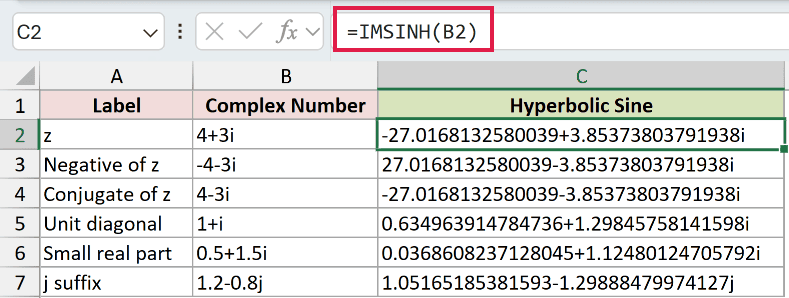
For 4+3i, C2 returns -27.0168132580039+3.85373803791938i. The real part is negative, even though both parts of the input are positive.

The next input, -4-3i, negates both parts. C3 returns 27.0168132580039-3.85373803791938i, reversing both signs in the answer too.

Negating the input negates its hyperbolic sine, a property called odd symmetry.

The conjugate input, 4-3i, changes only the imaginary sign. C4 returns -27.0168132580039-3.85373803791938i, so only the answer’s imaginary sign changes.

The last row uses 1.2-0.8j. Its result, 1.05165185381593-1.29888479974127j, keeps the lowercase j suffix.

These formulas calculate each row separately. Passing a bare range to IMSINH returns a single #VALUE! error, so copying down is the default method here.

Pro Tip: =IMSINH(+B2:B7) converts the range to an array with a unary plus. It spills in Excel 2021, Excel 2024 and Microsoft 365. In Excel 2019 and earlier, use the per-row formula above and copy it down.

Example 2: Compare IMSINH With SINH

A real input works in IMSINH, but the result’s data type still matters.

Below is the dataset. Column A contains real numbers, column B is for IMSINH results, and column C is for the real-number SINH comparison.

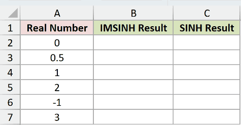
We want to compare the text returned by IMSINH with the numeric result from SINH.

Enter this formula in B2 and copy it down to B7:

=IMSINH(A2)

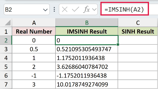
B2 displays 0, while B4 displays 1.1752011936438. Both are text results, even though neither contains an imaginary suffix.

For the real-number comparison, enter this SINH formula in C2 and copy it down to C7:

=SINH(A2)

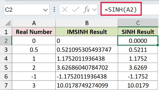
The SINH comparison displays 0.0000 in C2 and 1.1752 in C4. Its numeric format controls the displayed decimals.

For input 2, IMSINH displays 3.62686040784702, while the SINH comparison displays 3.6269.

Use SINH for real-number work. Keep IMSINH when your inputs can contain imaginary parts and you need complex results.

Pro Tip: Changing the number format won’t shorten complex text returned by IMSINH. Use IMREAL or IMAGINARY to extract a numeric component, or IMABS when you need the magnitude.

Example 3: Check the IMSIN Identity

You can check a hyperbolic sine by calculating it through complex sine.

Below is the dataset. Column A holds complex inputs; columns B:D are identity-check steps, E holds IMSINH results, and F is reserved for the numerical difference.

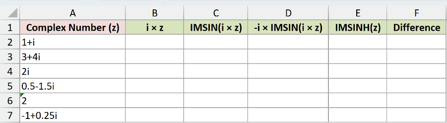
We want to verify the identity sinh(z) = -i × sin(i × z) against IMSINH.

For the first identity-check step, multiply the input by i in B2. Copy the formula down to B7:

=IMPRODUCT("i",A2)

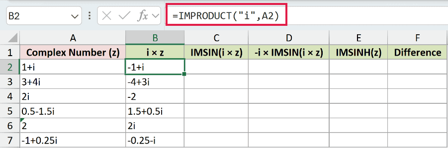
For 1+i, this check step returns -1+i in B2. IMPRODUCT handles the complex multiplication.

Next, calculate the sine of that check value in C2, then copy down to C7:

=IMSIN(B2)

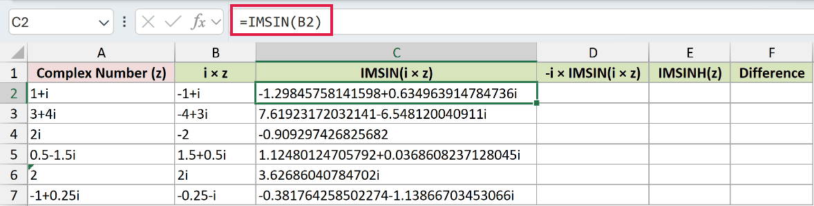
C2 returns -1.29845758141598+0.634963914784736i. This is an intermediate identity-check value, so there’s still a multiplication to complete.

Finish the identity-check route in D2, then copy down to D7:

=IMPRODUCT("-i",C2)

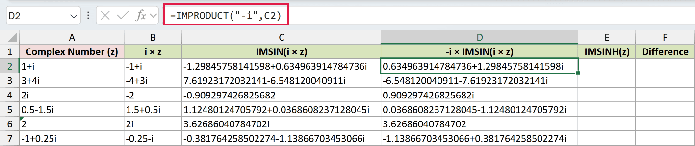
The completed identity check returns 0.634963914784736+1.29845758141598i in D2.

Now calculate the direct IMSINH answer in E2 and copy down to E7:

=IMSINH(A2)

E2 returns 0.634963914784736+1.29845758141598i, matching the completed identity check in D2.

Finally, calculate the numerical difference check in F2 and copy down to F7:

=IMABS(IMSUB(D2,E2))

How this check works:

IMSUB subtracts the direct IMSINH answer from the completed identity-check result.
IMABS returns the magnitude of that complex difference as a real number.
Every cell in F2:F7 displays 0.0E+00, confirming agreement for these inputs.

The pure imaginary input 2i returns 0.909297426825682i in E4. Its identity check in D4 agrees and also has no real part.

Columns B:D and F are checks, not additional answers to use. The direct IMSINH result is in column E.

Use a numerical difference when checking complex calculations. Comparing text strings can flag differences in the final digits even when the values are effectively equal.

Example 4: Diagnose Errors and Overflow

The size of the real part matters differently from the size of the imaginary part.

Below is the dataset. Column A describes each edge case, column B contains the input, and column C is reserved for results and deliberate error demonstrations.

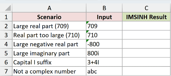
We want to distinguish numerical overflow from invalid complex-number text.

Enter this formula in C2 and copy it down to C7:

=IMSINH(B2)

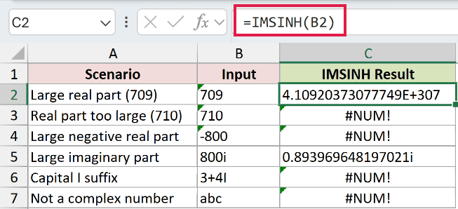
Each row teaches a different input check:

C2, input 709: Returns 4.10920373077749E+307. The result is extremely large, but Excel can still calculate it.
C3, input 710: Deliberately returns #NUM! because the real part causes overflow.
C4, input -800: Deliberately returns #NUM! too. A large negative real part can overflow as well.
C5, input 800i: Returns 0.893969648197021i. A large imaginary part doesn’t trigger the same overflow.
C6, input 3+4I: Deliberately returns #NUM! because the imaginary suffix is uppercase. Change it to lowercase i.
C7, input abc: Deliberately returns #NUM! because the text isn’t a complex number. Correct the source value.

The overflow boundary is a real-part magnitude of 710 or more in testing. Check which component is large before assuming every large complex input must fail.

Tips & Common Mistakes

Check empty inputs. IMSINH treats a blank referenced cell as zero and returns text 0. A missing input can therefore look like a valid answer.
Keep logical values out. TRUE or FALSE as the input returns #VALUE!. That differs from the #NUM! returned for invalid complex text.
Don’t blame spaces automatically. Excel accepted spaces within complex-number text in testing. Check the suffix and the structure of the input first.
Use complex-aware calculations. IMSINH results are text, so SUM over those cells won’t add the complex values. Extract the needed numeric components or use the appropriate complex-number function.
The exponential definition is another check. IMEXP, IMSUB and IMDIV can reproduce the hyperbolic sine through its exponential definition, although the final digits can differ.

You can now use IMSINH with complex inputs and check an answer through the sine identity.

When a result looks unexpected, check the input format and its real part before changing the formula.

List of All Excel Functions

Other Excel articles you may also like: