
The IMSQRT function in Excel returns the principal square root of a complex number as text.
IMSQRT also handles negative real numbers, returning complex square roots. That makes it useful when a quadratic equation has imaginary roots.
The principal root is the root whose real part is nonnegative. If you need the other root, you’ll calculate its negative separately.
I’ll show you how to handle negative inputs, find both square roots, and use IMSQRT to solve quadratic equations.
IMSQRT Function Syntax in Excel
IMSQRT takes one required argument:
=IMSQRT(inumber)
- inumber (required): The number whose square root you want. It can be a complex text value, a real number, or a cell reference containing either.
Complex text uses the form x+yi or x+yj. Use a lowercase i or j, and put quotation marks around complex text entered directly into a formula.
When to Use IMSQRT Function
- Calculate square roots of complex numbers stored in a worksheet column.
- Find imaginary square roots of negative real numbers.
- Obtain both square roots by negating the principal root.
- Solve quadratic equations whose discriminants are negative.
Example 1: Square Roots of Complex Numbers
Below is the dataset. Column A contains the complex inputs, and column B has the Square Root header and empty result cells.
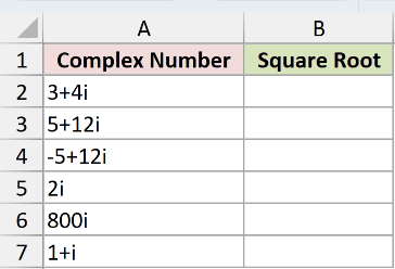
We want to calculate a square root for each input in column A.
Enter this formula in B2, then copy it down through B7:
=IMSQRT(A2)
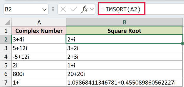
For 3+4i, the formula returns 2+i. The next input, 5+12i, returns 3+2i.
Purely imaginary inputs work too. The input 2i returns 1+i, while 800i returns 20+20i.
Some roots need longer decimals. For 1+i, B7 returns 1.09868411346781+0.455089860562227i.
These results are text, so changing the cell’s number format won’t shorten the decimal parts. We’ll handle that in the next example.
Passing a bare range to IMSQRT returns a single #VALUE! error. That’s why these examples calculate each row separately and copy the formula down.
Example 2: Negative Numbers and Rounding Noise
SQRT returns the square root of a nonnegative real number. Here, we compare it with IMSQRT to see how they handle negative inputs.
Below is the dataset. Column A contains real numbers; columns B through D reserve cells for the SQRT comparison, IMSQRT result, and cleaned result.
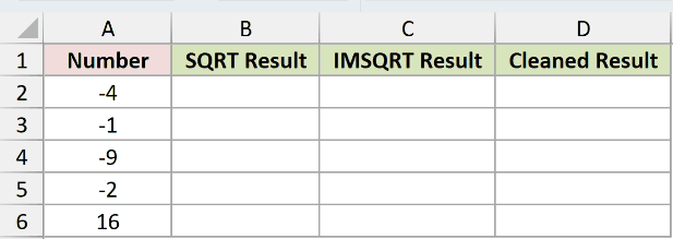
We want square roots of the negative inputs, then readable results without tiny rounding residues.
For the SQRT comparison, enter this formula in B2 and copy it down through B6:
=SQRT(A2)
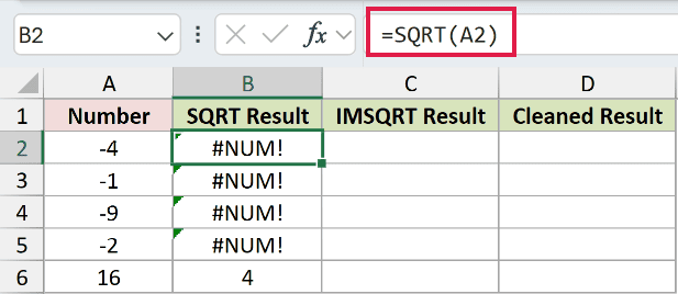
The SQRT comparison returns #NUM! for each negative input. Its final row returns 4 for the positive input 16.
Now enter the IMSQRT formula in C2 and copy it down through C6:
=IMSQRT(A2)
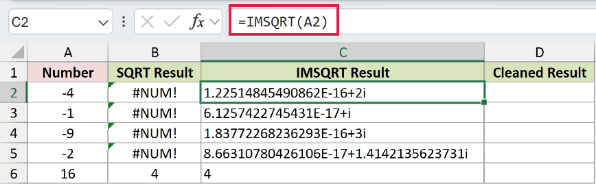
For -4, C2 returns 1.22514845490862E-16+2i. The raw text includes a tiny real part from floating-point rounding noise.
Likewise, -1 returns 6.1257422745431E-17+i. The scientific-notation fragments in these results represent small numerical residues.
For the cleanup, enter this formula in D2 and copy it down through D6:
=COMPLEX(ROUND(IMREAL(C2),10),ROUND(IMAGINARY(C2),10))
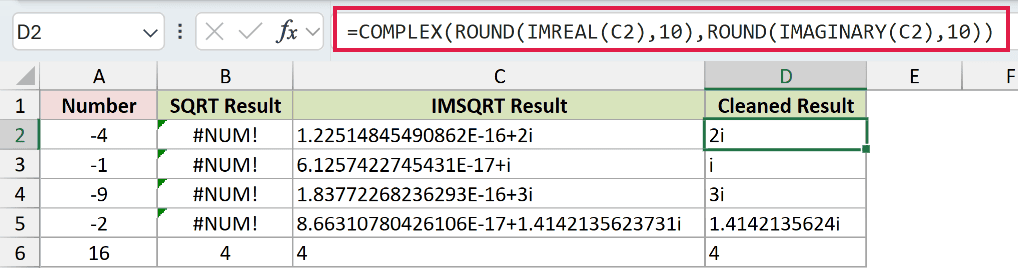
How this formula works:
- IMREAL extracts the real part of C2, and IMAGINARY extracts its imaginary part.
- ROUND rounds each extracted part to 10 decimal places.
- COMPLEX combines real and imaginary parts into complex text. Here, it rebuilds the IMSQRT result from the rounded parts.
The cleanup returns 2i, i, and 3i for the first negative inputs. For -2, the cleaned result is 1.4142135624i.
Pro Tip: Cleanup rounds the parts stored in the result. Keep the original IMSQRT result for calculations when you need its full precision, and use the rounded version for presentation.
Example 3: Find Both Square Roots
IMSQRT returns the principal root, but you may need its negative as well.
Below is the dataset. Column A holds complex inputs; columns B through D reserve cells for the principal root, other root, and squared check.
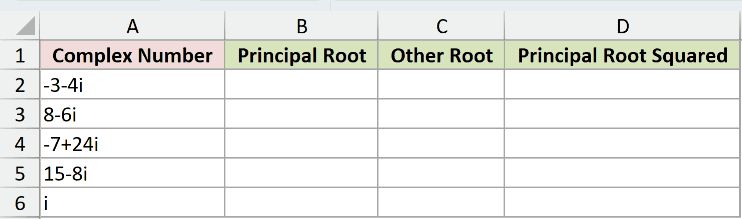
We want both roots and a check that squaring the principal root recovers the input.
Enter this formula in B2 and copy it down through B6:
=IMSQRT(A2)
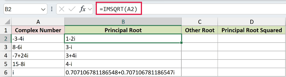
For -3-4i, B2 returns 1-2i. Its real part is positive, even though its imaginary part is negative.
To calculate the other root, enter this formula in C2 and copy it down through C6:
=IMPRODUCT(B2,-1)
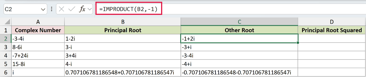
IMPRODUCT multiplies the complex root by -1, reversing both signs. C2 returns -1+2i, the other square root of -3-4i.
For the squared check, enter this formula in D2 and copy it down through D6:
=IMPRODUCT(B2,B2)
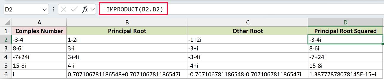
D2 returns -3-4i, matching the original input. The next row returns 8-6i after squaring its principal root, 3-i.
The i row needs closer attention: D6 returns 1.38777878078145E-15+i. That E-15 real part is rounding noise from squaring an approximate root.
So the squared check can recover the input with a tiny numerical residue. Don’t expect every returned text string to match its input exactly.
Example 4: Solve Quadratic Equations
Below is the dataset. Column A lists equations, B through D contain their coefficients, and E through G reserve cells for the discriminant and roots.
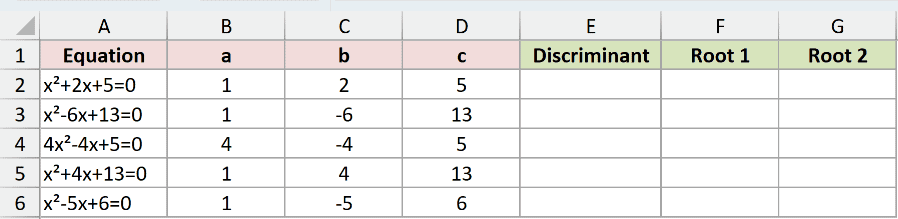
We want both solutions for each equation, including those with a negative discriminant.
Calculate the discriminant in E2, then copy this formula down through E6:
=C2^2-4*B2*D2
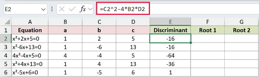
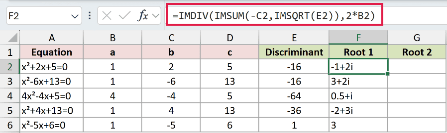
Columns B, C, and D hold coefficients a, b, and c. For x²+2x+5=0, the discriminant in E2 is -16.
Calculate the first root in F2, then copy this formula down through F6:
=IMDIV(IMSUM(-C2,IMSQRT(E2)),2*B2)
How this formula works:
- IMSQRT calculates the square root of the discriminant in E2, including when it’s negative.
- IMSUM adds that complex root to the negated coefficient from C2.
- IMDIV divides the complex numerator by twice the coefficient in B2.
F2 returns -1+2i. The tiny real-part noise introduced by the negative discriminant’s square root disappears after the IMSUM and IMDIV calculations here.
For the second root, enter this formula in G2 and copy it down through G6:
=IMDIV(IMSUB(-C2,IMSQRT(E2)),2*B2)
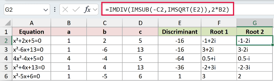
IMSUB subtracts complex numbers. Here, it subtracts the discriminant’s square root from the negated coefficient in C2 to find the second root. G2 returns -1-2i.
For 4x²-4x+5=0, the roots are 0.5+i and 0.5-i. Both formulas use the coefficients from their own row.
The real-root equation x²-5x+6=0 also works. Its discriminant is 1, and the root formulas return 3 and 2, still as text.
Example 5: Accepted Inputs and Deliberate Errors
A valid-looking input can fail because of its suffix or data type.
Below is the dataset. Column A labels each input type, column B holds the test inputs, and column C reserves cells for roots or deliberate errors.
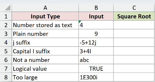
We want to distinguish accepted inputs from errors that need correction.
Enter this formula in C2 and copy it down through C8:
=IMSQRT(B2)
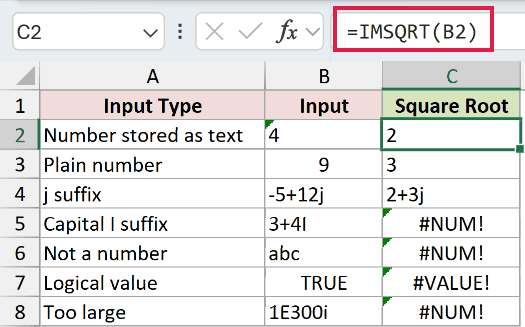
The text number 4 returns 2, and the plain number 9 returns 3. Both are valid inputs.
The input -5+12j returns 2+3j. IMSQRT preserves the lowercase j suffix.
The remaining rows show deliberate errors:
C5, capital suffix:3+4Ireturns#NUM!. Change the uppercase suffix to lowercasei.C6, invalid text:abcreturns#NUM!because it doesn’t represent a number. Correct the source input.C7, logical value: TRUE returns#VALUE!. Supply the intended numeric or complex input instead of a logical value.C8, oversized input:1E300ireturns#NUM!in testing.
Tips & Common Mistakes
- Keep complex results in complex arithmetic. IMSQRT returns text, so use functions such as IMSUM, IMSUB, IMPRODUCT, and IMDIV for subsequent calculations.
- Check empty source cells. In testing, a blank cell returned the text
0. A missing input can therefore look like a calculated answer. - Don’t assume spaces cause an error. Spaces inside complex text were tolerated in testing. Check the suffix and actual contents before blaming spacing.
- IMABS returns a complex number’s magnitude, its distance from zero. To check the IMSQRT result, compare
IMABS(IMSQRT(z))withSQRT(IMABS(z)). They are equal;zis the complex input. - Treat rounding as a precision choice. The cleanup in Example 2 is useful for readable output, but rounding can also remove a small component.
Related Excel Functions / Articles:
