
The PHI function in Excel returns the height of the standard normal bell curve at a given value. That height is called a probability density.
A density describes the curve at a point. To find a probability, you need an area under the curve across an interval, rather than its height alone.
In this article, I’ll show you how to calculate curve heights, estimate probabilities over narrow bands, and scale PHI results to match real measurements and histogram counts.
PHI Function Syntax in Excel
PHI takes a single required argument:
=PHI(x)
- x (required): The value where you want the standard normal curve’s height. You can supply a number, a cell reference, or a range of values.
Here, x is a z value: a measurement’s distance from its mean, expressed in standard deviations. Negative values sit below the mean; positive values sit above it.
When to Use PHI Function
- Generate curve heights for a list of z values when preparing a bell-curve chart.
- Estimate the probability within a narrow band by multiplying its width by the curve height at its center.
- Calculate density for measurements such as heights after adjusting for their mean and standard deviation.
- Estimate counts for histogram bins so you can compare observed data with a normal model.
Example 1: Calculate Standard Normal Curve Heights
Let’s start with a list of values on either side of the curve’s center.
Below is the dataset. Column A contains z values, and the green result column B will hold the corresponding curve heights.
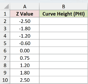
We want to calculate the height of the standard normal curve at every z value.
Here is the formula to enter in B2:
=PHI(A2:A10)
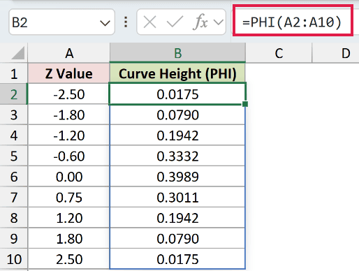
The formula returns a result for each input and spills into B2:B10. You enter it in B2 only.
These range formulas spill in Excel 2021, Excel 2024, and Microsoft 365. In Excel 2019 and earlier, use a single-cell reference and copy the per-row formula down.
At the center, A6 contains 0.00 and B6 displays 0.3989, the peak height. For the z value 0.75, B7 displays 0.3011.
The matching results on opposite sides show the curve’s symmetry. Both -1.20 and 1.20 return 0.1942, while -2.50 and 2.50 return 0.0175.
As you move farther from the center, the curve becomes lower. These results describe heights, not the probability of getting each exact z value.
Example 2: Estimate Probability Across a Band
Now let’s give those curve heights a width so they describe an area.
Below is the dataset. Columns A and B contain band centers and widths; columns C and D will show the PHI estimate and exact probability.
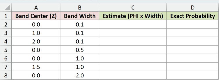
We want to estimate the probability within each band, then check how closely the estimate matches the actual area under the curve.
Here is the formula to enter in C2:
=PHI(A2:A8)*B2:B8
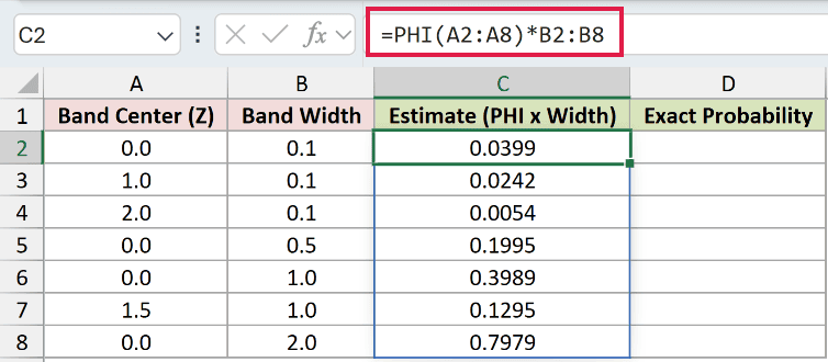
PHI calculates each band’s center height. Multiplying by its width estimates the area as a rectangle, and the results spill into C2:C8.
For the band centered at 0.0 with width 0.1, the estimate is 0.0399. Widening the band to 2.0 produces an estimate of 0.7979.
To check the approximation, we’ll use NORM.S.DIST. With TRUE, it returns the cumulative probability up to a z value, letting us calculate each band’s area.
Enter this comparison formula in D2:
=NORM.S.DIST(A2:A8+B2:B8/2,TRUE)-NORM.S.DIST(A2:A8-B2:B8/2,TRUE)
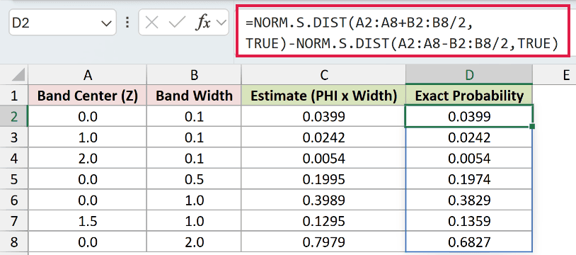
The formula finds each band’s upper and lower edges by adding or subtracting half its width. Subtracting the cumulative probabilities leaves the area between those edges.
The exact probabilities spill into D2:D8. For the narrow band in the first row, both columns display 0.0399.
For the width of 0.5 centered at 0.0, the PHI estimate is 0.1995, compared with 0.1974 in the exact column.
For the wider band in the last row, the estimate is 0.7979, compared with an exact probability of 0.6827.
The rectangle uses the center’s height across the entire width. Around the peak, that overstates the area because the curve falls away on either side.
For the band centered at 1.5 with width 1.0, PHI underestimates the area. Its estimate is 0.1295, compared with the exact probability of 0.1359.
Pro Tip: Treat PHI multiplied by width as an approximation. When you need the probability across a band, use the cumulative-probability difference shown in column D.
Example 3: Calculate Density in Real Units
Next, let’s use PHI with measurements in inches instead of z values.
Below is the dataset. Column A lists adult heights, while the card in E:F holds the assumed mean and standard deviation for the normal model.
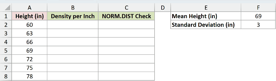
We want the density per inch at each height, using the mean of 69 inches and standard deviation of 3 inches.
STANDARDIZE converts each height into its distance from the mean in standard deviations. That gives PHI the z values it needs.
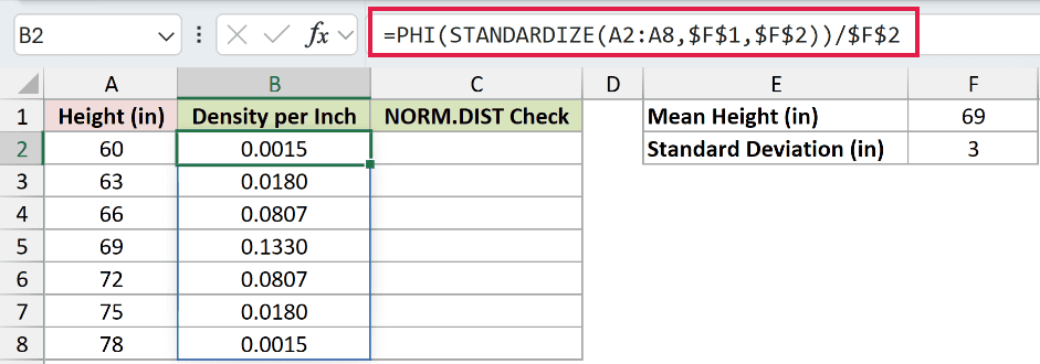
Here is the formula to enter in B2:
=PHI(STANDARDIZE(A2:A8,$F$1,$F$2))/$F$2
How this formula works:
- STANDARDIZE subtracts the mean in
$F$1from each height and divides by the standard deviation in$F$2. - PHI returns the standard normal curve height at each standardized value.
- Dividing that result by
$F$2converts the density from the z scale to density per inch.
The results spill into B2:B8. At 69 inches, the density is 0.1330. At both 66 and 72 inches, it is 0.0807.
The final division matters. Standardizing the input changes the horizontal scale; dividing PHI’s result by the standard deviation adjusts the vertical scale to match.
For a check, NORM.DIST calculates normal density directly from a measurement, mean, and standard deviation. Its FALSE argument requests density, matching what our PHI formula calculates.
Enter the comparison formula in C2:
=NORM.DIST(A2:A8,$F$1,$F$2,FALSE)
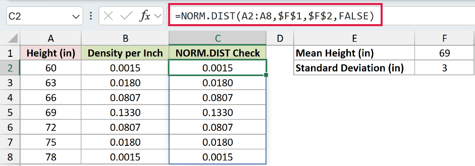
The check spills into C2:C8 and matches the PHI-based results throughout. For example, both columns display 0.0015 at 60 inches and 0.0180 at 63 inches.
NORM.DIST is shorter for this task. The PHI version shows the separate steps needed to move between a standard normal curve and your measurement scale.
Example 4: Estimate Histogram Counts With PHI
Finally, let’s scale the curve so its heights can be compared with counts of recorded days.
Below is the dataset. Columns A and B contain mileage-bin midpoints and actual day counts; the E:F card holds the tracking total, mean, standard deviation, and bin width.
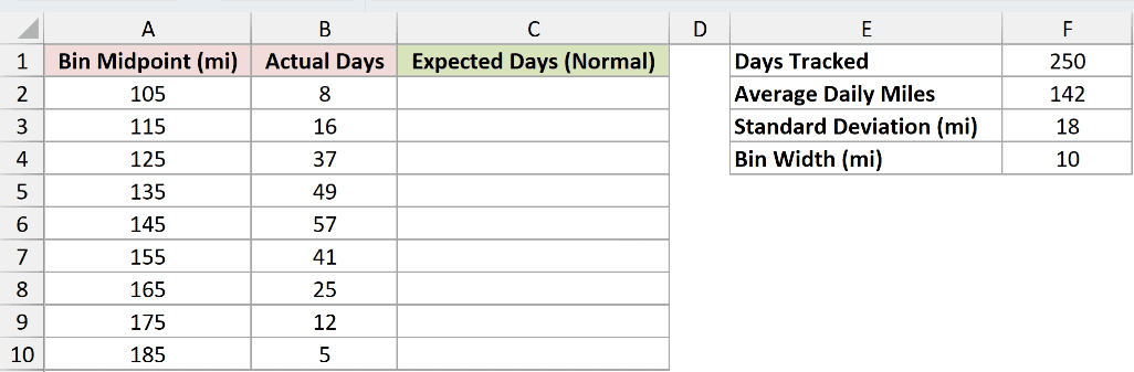
We want to estimate how many days fall in each mileage bin under a normal model.
The card specifies 250 tracked days, an average of 142 miles, a standard deviation of 18 miles, and a bin width of 10 miles.
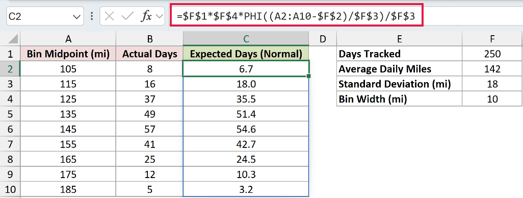
Here is the formula to enter in C2:
=$F$1*$F$4*PHI((A2:A10-$F$2)/$F$3)/$F$3
How this formula works:
- Subtracting
$F$2and dividing by$F$3converts each bin midpoint into a z value. - PHI calculates the standard normal curve height, and the final division by
$F$3converts it to density per mile. - Multiplying by the bin width in
$F$4estimates the probability within that bin. - Multiplying by the tracked days in
$F$1converts the probability estimate into an expected count.
The results spill into C2:C10. At the 145-mile midpoint, the model estimates 54.6 days, compared with 57 actual days.
At the 105-mile midpoint, it estimates 6.7 days, compared with 8 actual days. These are model estimates, so fractional day counts are appropriate.
This scales PHI’s curve heights to the same count scale as the histogram.
Pro Tip: These expected counts use the midpoint approximation from Example 2. Wider bins can make that approximation less accurate because the density changes within each bin.
Tips & Common Mistakes
- PHI is available in Excel 2013 and later.
- A blank input cell is treated as zero, so it produces the curve’s center height rather than a missing result. Check for blanks before interpreting your results.
- Ordinary text such as
applereturns#VALUE!. Numeric text and logical values can be converted silently, so an error-free result doesn’t prove the input was a measurement. - Keep probability and density separate. PHI returns a height; a probability requires an area across a band, as shown in Example 2.
- When converting PHI results to density in the original measurement units, keep the final division by the standard deviation. Standardizing the input alone doesn’t complete that conversion.
Related Excel Functions / Articles:
