
The PRICEMAT function in Excel returns the price per $100 face value of a security that pays its interest at maturity.
For a certificate of deposit (CD) bought after issue, that price depends on the original interest rate, your required annual yield, and the dates involved.
PRICEMAT returns a clean price, which excludes interest already accrued before settlement. You’ll need to add that interest when calculating the cash paid to the seller.
In this article, I’ll show you how to price CDs, compare prices at different yields, and turn a quoted price into cash at settlement.
PRICEMAT Function Syntax in Excel
PRICEMAT takes the security’s dates, interest rate, annual yield, and an optional day-count basis:
=PRICEMAT(settlement, maturity, issue, rate, yld, [basis])
- settlement (required): The date the purchase settles and the buyer takes ownership.
- maturity (required): The date the security matures and pays its interest.
- issue (required): The date the security was originally issued.
- rate (required): The annual interest rate set at issue.
- yld (required): The annual yield used to calculate the price.
- basis (optional): The convention used to count days. If omitted, Excel uses the US (NASD) convention. Use the convention specified for the security.
The interest rate describes what the security pays. The yield describes the return used to value it at settlement.
When to Use PRICEMAT Function
- Price a CD that pays all its interest at maturity and is being purchased after issue.
- Calculate prices for a watchlist using each security’s dates, rates, and day-count basis.
- See how a change in required yield affects the same security’s price.
- Calculate cash at settlement by adding accrued interest and scaling the quote to the face amount.
Example 1: Price a CD Bought After Issue
Let’s start with a CD that pays all its interest at maturity.
Below is the dataset. Cells B1:B6 contain the dates, interest rate, annual yield, and basis. The labeled cells beneath them will hold the price and yield check.
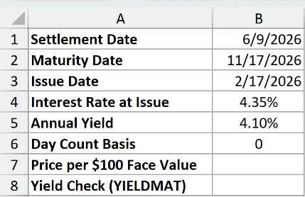
We want the price per $100 face value using the required annual yield in B5.
Enter this formula in B7:
=PRICEMAT(B1,B2,B3,B4,B5,B6)
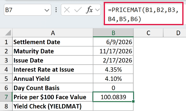
The result is 100.0839. This is a quote per $100 face value, so the CD has a small premium above face value.
The formula reads settlement from B1, maturity from B2, and issue from B3. Keep that order even though issue comes first chronologically.
Here, the original interest rate is 4.35%, while the required annual yield is 4.10%. PRICEMAT uses both to calculate the price.
We can check that price with YIELDMAT, which calculates annual yield from a maturity-interest security’s price. Feeding it the PRICEMAT result should recover our original yield.
Enter this check in B8:
=YIELDMAT(B1,B2,B3,B4,B7,B6)
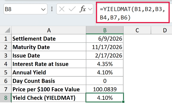
The check returns 4.10%, matching B5. It uses the calculated price in B7 while keeping the dates, interest rate, and basis unchanged.
Example 2: Price a Watchlist of CDs
Now let’s calculate prices for a sample watchlist of CDs that all pay interest at maturity.
Below is the dataset. Column A identifies each CD, B:D hold dates, E:F hold rates, and G holds the basis. Column H will show prices.

We want a price for each CD using the inputs on its own row.
Enter this formula in H2:
=PRICEMAT(+B2:B7,+C2:C7,+D2:D7,+E2:E7,+F2:F7,+G2:G7)
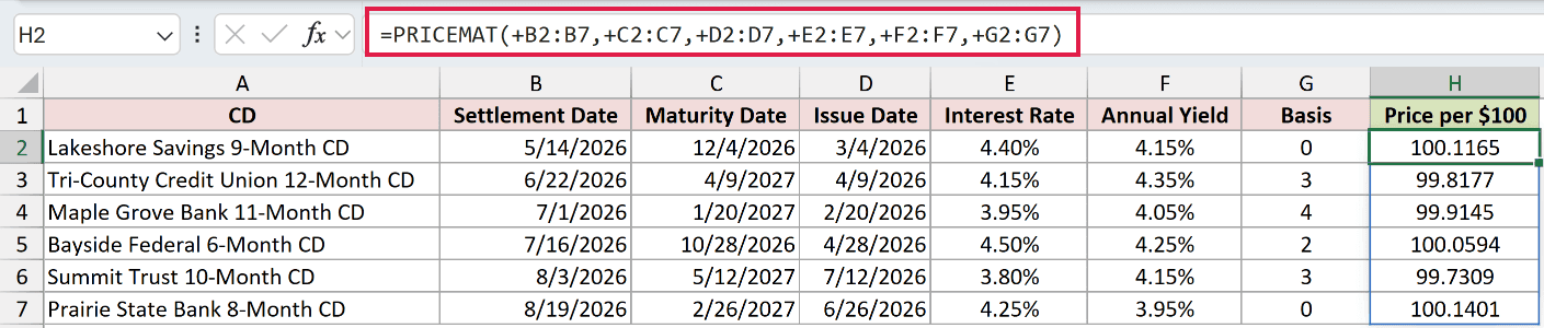
The plus sign before each range turns its cell references into values PRICEMAT can process together. Without it, a bare range returns a single #VALUE! error.
The formula spills into H2:H7 in Excel 2021, Excel 2024, and Microsoft 365. Each price stays aligned with its CD.
In Excel 2019 and earlier, use a per-row formula copied down, as shown in Example 5.
Lakeshore Savings returns 100.1165, while Tri-County Credit Union returns 99.8177. The former is above face value; the latter is below it.
Maple Grove Bank returns 99.9145, Bayside Federal returns 100.0594, Summit Trust returns 99.7309, and Prairie State Bank returns 100.1401.
Each row uses its own basis from column G. Keep that input tied to the security’s terms when you reuse the watchlist.
Example 3: Compare Prices at Different Yields
Next, let’s change the required yield while keeping the CD itself unchanged.
Below is the dataset. A2:A6 contain annual yield scenarios. The card in D:E holds the CD’s dates, interest rate, and basis. Column B will hold prices.
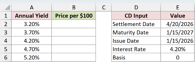
We want to see how each yield changes the price of this same CD.
Enter this formula in B2:
=PRICEMAT($E$2,$E$3,$E$4,$E$5,+A2:A6,$E$6)
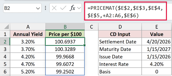
The absolute references keep the CD inputs fixed. Only the yield changes, and the prices spill into B2:B6.
At 3.20%, the price is 100.6937. At 5.20%, it falls to 99.2502. A higher required yield means a lower price for this fixed payout.
Both the interest rate and yield are 4.20%, but PRICEMAT returns 99.9668, slightly below face value.
Even with matching rates, the price depends on dates because PRICEMAT discounts the maturity payment from settlement and subtracts interest accrued since issue.
Example 4: Calculate Cash Paid at Settlement
A clean price isn’t the full cash amount you pay when the security has already accrued interest.
Below is the dataset. B1:B6 contain the CD inputs, and B7 holds the face amount. The labeled rows below will calculate price, accrued interest, and settlement cash.
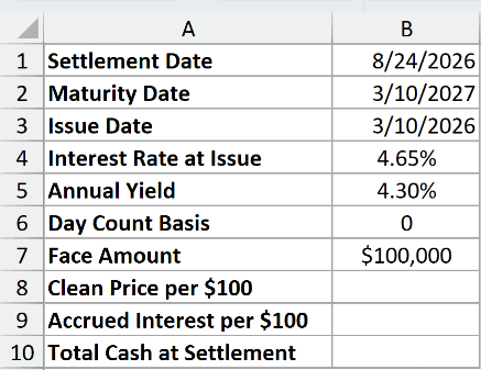
We want the cash at settlement for a $100,000 face amount, including the seller’s accrued interest.
First, calculate the clean price in B8:
=PRICEMAT(B1,B2,B3,B4,B5,B6)
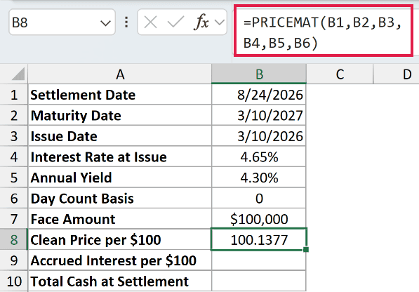
PRICEMAT returns 100.1377 per $100 face value. This excludes the interest earned between issue and settlement.
ACCRINTM calculates accrued interest for a security that pays interest at maturity. Here, it calculates the amount we need to add to PRICEMAT’s clean price.
Enter this formula in B9:
=ACCRINTM(B3,B1,B4,100,B6)
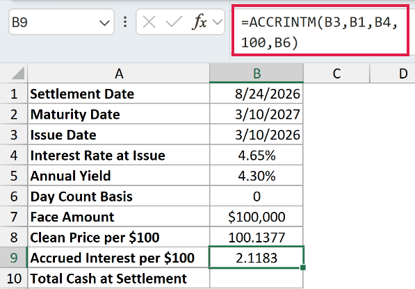
The result is 2.1183 per $100 face value. B3 supplies the issue date, while B1 supplies settlement as the endpoint for this accrued-interest calculation.
The literal 100 keeps accrued interest on the same scale as the PRICEMAT quote. B4 and B6 supply the original interest rate and basis.
Now calculate the total cash in B10:
=(B8+B9)*B7/100
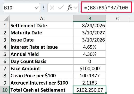
The result is $102,256.07. The formula adds clean price and accrued interest, then scales their combined amount to the face value in B7.
Pro Tip: Reference B8 and B9 directly when calculating settlement cash. This keeps their stored precision instead of calculating from the rounded figures displayed on the sheet.
Example 5: Diagnose PRICEMAT Input Errors
Finally, let’s look at input problems that PRICEMAT flags.
Below is the dataset. Column A names each scenario, B:G contain its inputs, and H will show the result. The invalid rows are deliberate demonstrations.

We want to identify which input causes each error so we can correct the source cell.
Enter this formula in H2, then copy it down through H7:
=PRICEMAT(B2,C2,D2,E2,F2,G2)
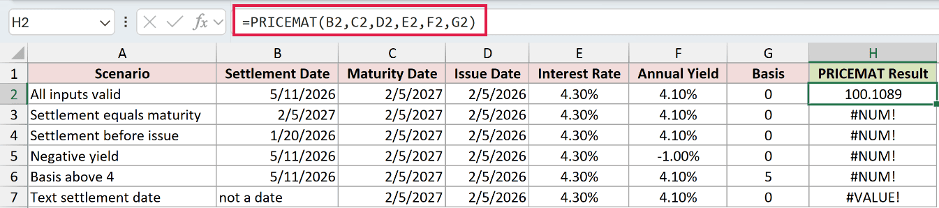
This example uses separate row formulas so you can inspect each invalid case in the formula bar.
H2returns 100.1089: This is the valid comparison row.H3returns#NUM!: Settlement equals maturity. Check the dates and use a settlement date before maturity.H4returns#NUM!: Settlement is before issue. Correct the date order; Excel rejects this case.H5returns#NUM!: The annual yield is -1.00%. Check the yield input and replace the negative value.H6returns#NUM!: The basis is 5, which is invalid. Select the valid convention required by the security.H7returns#VALUE!: The settlement cell contains not a date. Replace it with a real Excel date.
The error results in H3:H7 aren’t usable prices, even though they sit beneath the same result header as the valid calculation.
In testing, a cell containing the text 5/11/2026 was accepted as a date, so text doesn’t always trigger an error.
That silent conversion can depend on regional settings. Use real Excel date cells so a readable-looking date doesn’t get interpreted differently on another computer.
Tips & Common Mistakes
- Check the payment pattern. These examples assume all interest is paid at maturity. Confirm that this matches the security before using PRICEMAT.
- Keep rate and yield separate. The original interest rate stays with the security. The annual yield is the return you’re using to calculate its price at settlement.
- Enter rates as percentages. In Example 1, the interest-rate cell contains
4.35%. Keep the percentage sign when replacing that input. - Zero yield is allowed. Testing confirmed that PRICEMAT accepts it. Don’t treat zero yield as the same error as negative yield.
- Use a whole-number basis code. Testing confirmed that
3.9is truncated to3. A decimal code won’t preserve a separate convention. - Separate quote from payment. The PRICEMAT result is per $100 face value and excludes accrued interest. Use Example 4’s calculation when you need settlement cash.
Keep the settlement date and accrued-interest calculation together when reusing the workbook. Changing the purchase date affects both the clean price and the amount paid to the seller.
Other Excel articles you may also like:
