Highlight Entire Row Based on Cell Value in Excel

If you want Excel to color a whole row when one cell in it has a certain value, like every order marked Overdue, conditional formatting can do it for you.

The catch is that the quick Highlight Cells Rules only color the cell that matches.

To light up the entire row, you need a formula rule with one small dollar sign in the right place.

In this article, I’ll show you six ways to do it, from a basic formula rule to SEARCH, AND, color-coded statuses, a drop-down picker, and filter-and-fill.

Method #1: Using a Conditional Formatting Formula Rule

This is the method I’d use in most cases. You write one short formula. Excel checks it for every row and colors the rows where it’s TRUE.

Below I have a task list with the Task ID, Task, Owner, Priority, Hours, and Status for 10 tasks. I want to highlight every row where the Status is Blocked.

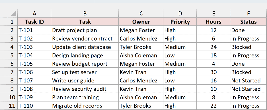
Here are the steps to highlight the rows:

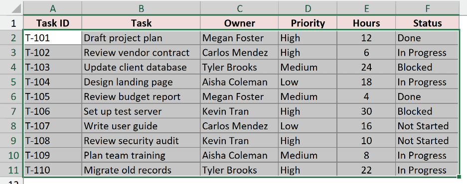
1. Select the data without the headers (A2:F11 here). Start the selection from cell A2, so it stays the active cell.

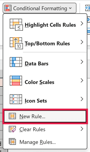
2. On the Home tab, click Conditional Formatting, then click New Rule.

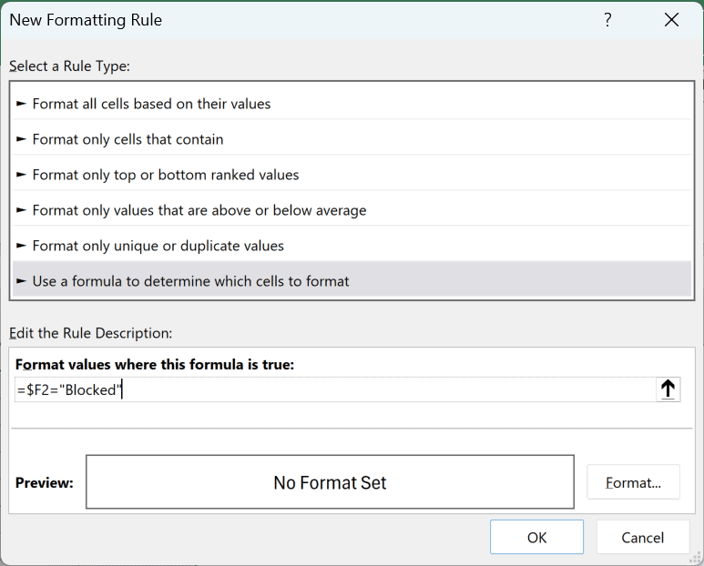
3. In the New Formatting Rule dialog box, choose Use a formula to determine which cells to format. In the formula box, enter the formula below.

=$F2="Blocked"

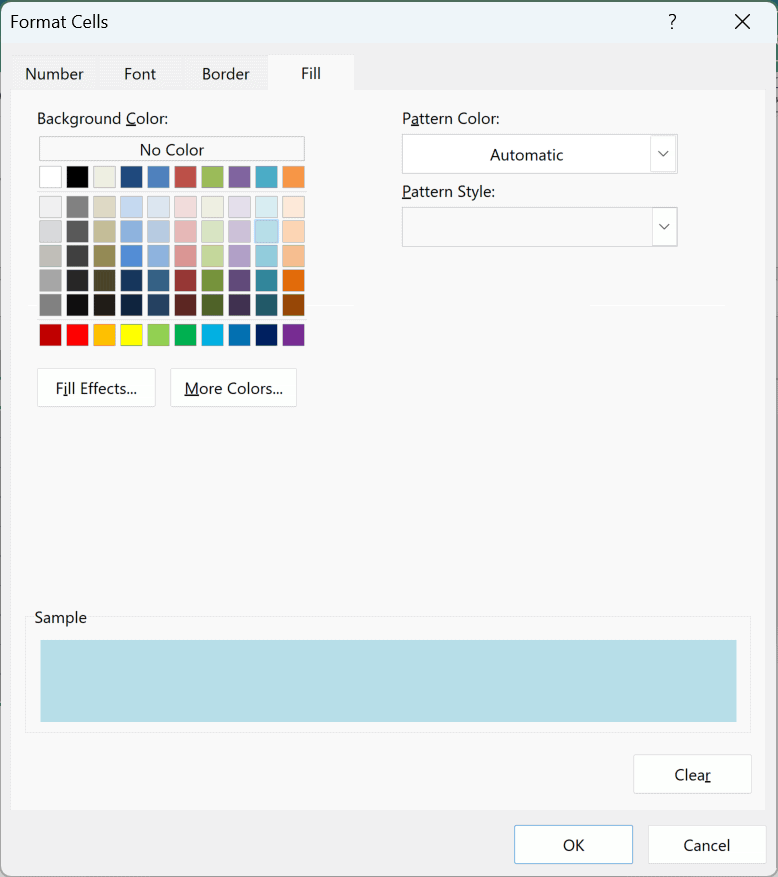
4. Click the Format button. On the Fill tab, pick a light blue color from the palette and click OK.

5. Click OK to close the New Formatting Rule dialog box.

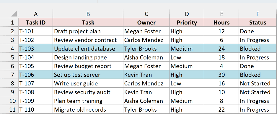
The two Blocked tasks, T-103 and T-106, are now highlighted across the whole row, from Task ID to Status.

How does this formula work?

Excel writes the formula for the active cell (A2) and then adjusts it for every other cell in the selection, just like copying a formula.

The dollar sign in $F2 locks the column but not the row. So every cell in row 2 checks F2, every cell in row 3 checks F3, and so on.

That’s why the whole row changes color together. When the Status in column F says Blocked, all six cells in that row get the fill.

Without the dollar sign, the formula =F2=”Blocked” shifts one column for each cell.

Only the Task ID cells in column A would check the Status column, so only column A would light up.

Note: If you click a cell while typing in the formula box, Excel inserts it as $F$2, which locks the row too. Then every row checks F2 and nothing lines up. Press F4 until it reads $F2.

The same rule works with numbers. Swap the text check for a comparison.

For example, to highlight every task that needs more than 20 hours, use this formula in the same steps:

=$E2>20

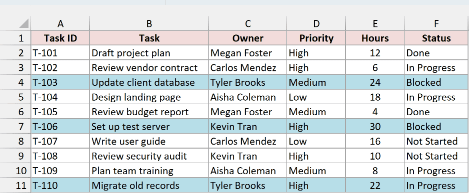
Three rows light up this time: T-103 (24 hours), T-106 (30 hours), and T-110 (22 hours).

You can use any comparison here, such as >=, <, or <> (not equal to).

Method #2: Using SEARCH for a Partial Text Match

Sometimes the cell won’t be an exact match. You want the row highlighted when the cell contains a word somewhere inside it.

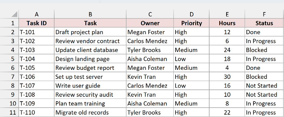
Below I have the same task list. This time I want to highlight every task that has the word “review” in its name.

Here are the steps to highlight the rows:

1. Select A2:F11, starting from A2.
2. On the Home tab, click Conditional Formatting, then New Rule.
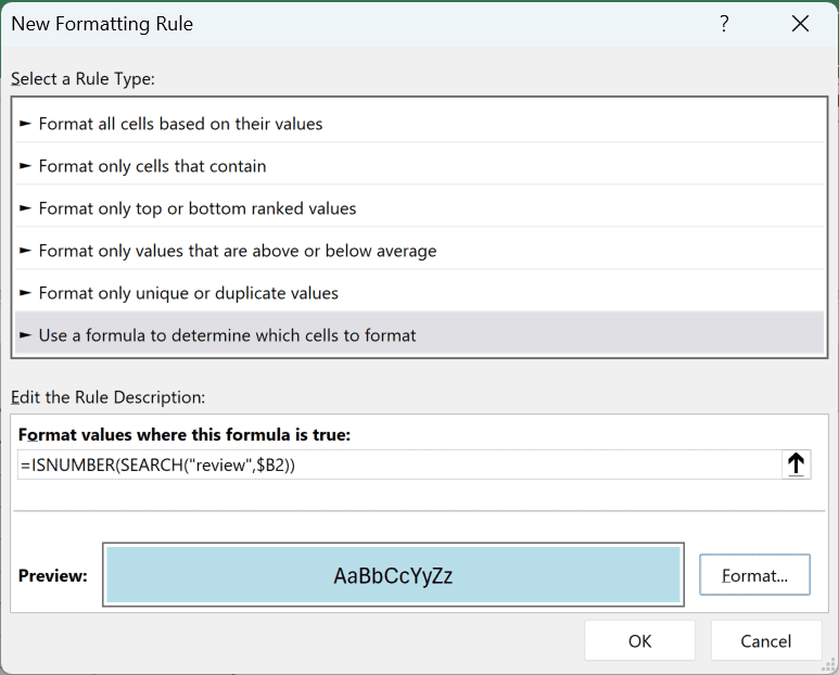
3. Choose Use a formula to determine which cells to format and enter the formula below.
4. Click Format, pick a fill color on the Fill tab, and click OK twice.

=ISNUMBER(SEARCH("review",$B2))

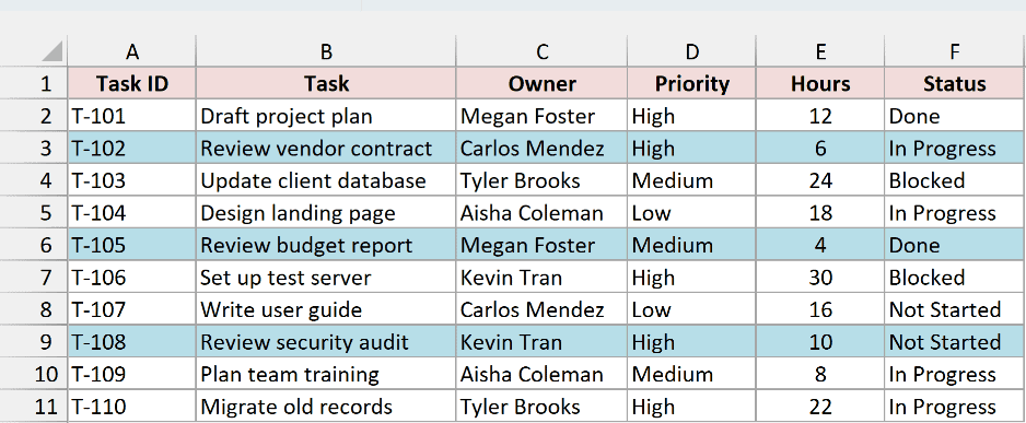
Excel highlights T-102, T-105, and T-108, the three tasks that start with “Review”.

How does this formula work?

SEARCH looks for “review” inside the task name in column B. If it finds the word, it returns its position as a number. If not, it returns a #VALUE! error.

ISNUMBER turns that into TRUE or FALSE. A number means the word is there, so the row gets the fill. An error means it isn’t, so the row stays plain.

SEARCH doesn’t care about case, so “Review”, “review”, and “REVIEW” all count. It also matches the word anywhere in the cell, not just at the start.

Method #3: Using AND for Multiple Conditions

If one condition isn’t enough, you can check two or more columns in the same rule.

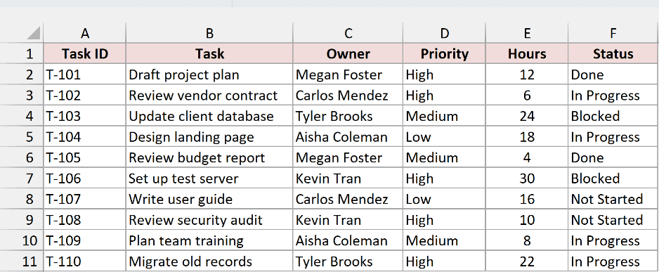
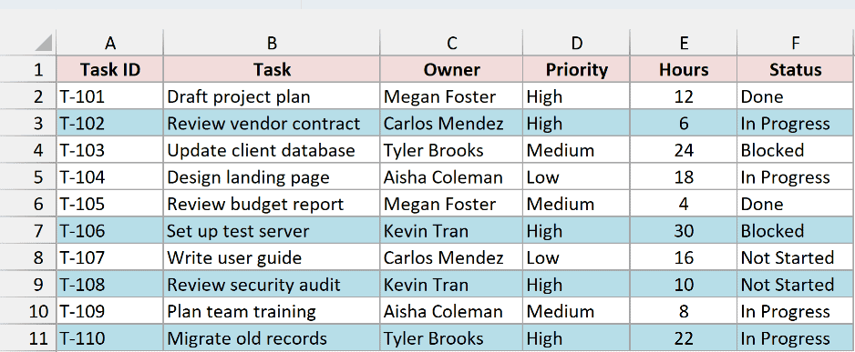
Below I have the same task list. I want to highlight the tasks that are High priority and not yet Done, since those need attention first.

Here are the steps to highlight the rows:

1. Select A2:F11, starting from A2.
2. On the Home tab, click Conditional Formatting, then New Rule.
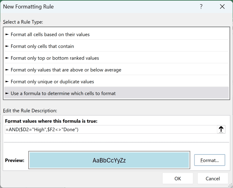
3. Choose Use a formula to determine which cells to format and enter the formula below.
4. Click Format, pick a fill color on the Fill tab, and click OK twice.

=AND($D2="High",$F2<>"Done")

Four rows get highlighted: T-102, T-106, T-108, and T-110. T-101 is also High priority, but it’s already Done, so it’s left alone.

How does this formula work?

AND returns TRUE only when every condition inside it is TRUE. Here, the Priority in column D has to be High, and the Status in column F can’t be Done.

Both references have the dollar sign before the column letter, so each row checks its own Priority and Status.

If you want a row highlighted when either condition is true, use OR instead of AND, as in =OR($D2=”High”,$F2=”Blocked”).

Method #4: Using Separate Rules for Different Colors

A single rule gives you one color. If you want each status to get its own color, you create one rule per status.

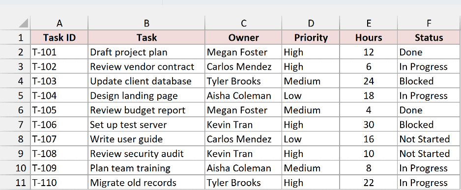
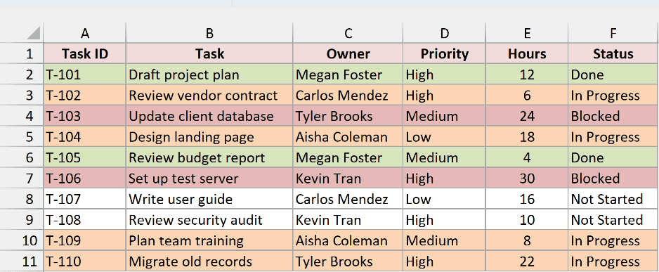
Below I have the same task list. I want Done rows in green, In Progress rows in orange, and Blocked rows in red.

Here are the steps to set up the rules:

1. Select A2:F11, starting from A2.
2. Go to Home > Conditional Formatting > New Rule, choose Use a formula to determine which cells to format, and enter =$F2=”Done”.
3. Click Format, pick a light green fill, and click OK twice.
4. With the same range still selected, repeat steps 2 and 3 with =$F2=”In Progress” and a light orange fill.
5. Repeat them once more with =$F2=”Blocked” and a light red fill.

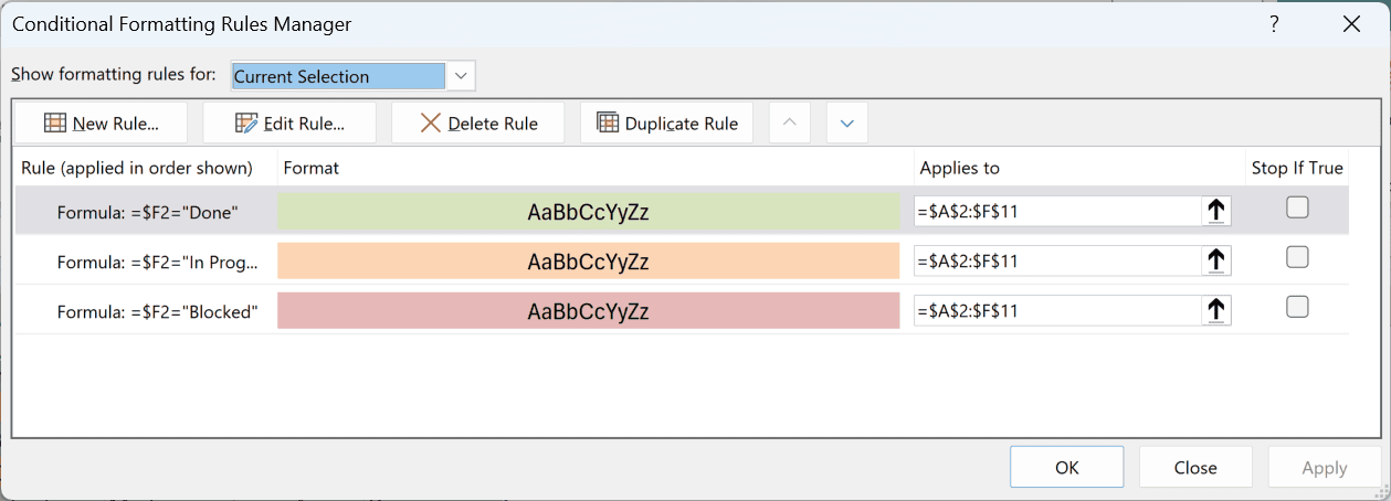
To check your work, go to Home > Conditional Formatting > Manage Rules. You’ll see all three rules, each applied to $A$2:$F$11.

Every row now picks up the color of its status. The two Not Started tasks have no rule, so they stay white.

Note: If two rules can be TRUE for the same row, the one higher in the Manage Rules list wins the fill. Use the up and down arrows there to change the order.

Method #5: Using a Drop-Down to Pick the Value

Instead of typing the value into the rule, you can point the rule at a cell. Then you change the cell, and the highlighted rows change with it.

Below I have the same task list.

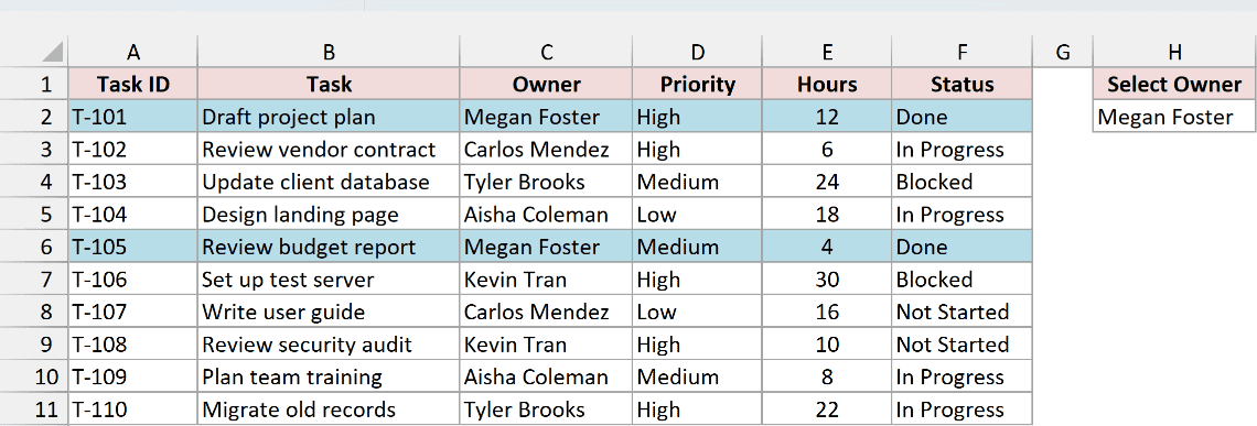
Next to it, cell H2 holds an owner’s name under a Select Owner label, and I want to highlight all tasks for that owner.

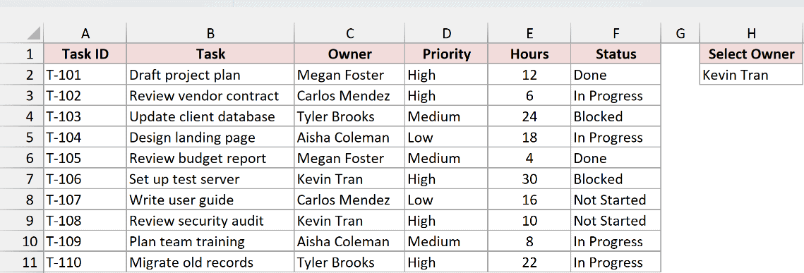
First, turn H2 into a drop-down list, so you can pick a name instead of typing it:

1. Select cell H2. On the Data tab, click Data Validation. In the Allow box, choose List, type the owner names in the Source box separated by commas, and click OK.

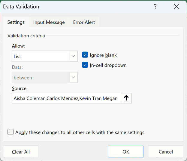
Now create the rule that reads H2:

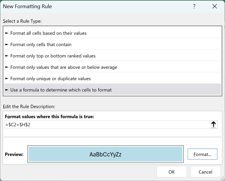
2. Select A2:F11, starting from A2. Go to Home > Conditional Formatting > New Rule, choose Use a formula to determine which cells to format, and enter the formula below. Set a fill color and click OK twice.

=$C2=$H$2

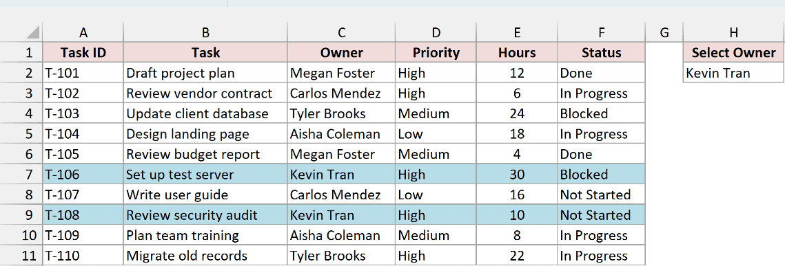
With Kevin Tran selected in H2, his two tasks (T-106 and T-108) are highlighted.

Now pick Megan Foster from the drop-down. The highlight moves to her tasks, T-101 and T-105, without touching the rule.

How does this formula work?

$C2 is the Owner in each row, locked to column C like before. $H$2 has dollar signs on both parts, so every row compares its owner against the same cell.

If you forget the second dollar sign and write $H2, row 3 would check H3, row 4 would check H4, and so on.

Those cells are empty, so only row 2 could ever match.

Method #6: Using Filter and Fill Color

If you just need to color some rows once, say before you send a file to someone, you don’t need a rule at all.

A filter and the Fill Color button do the job.

Keep in mind this is a one-time fill. If the values change later, the colors won’t follow them.

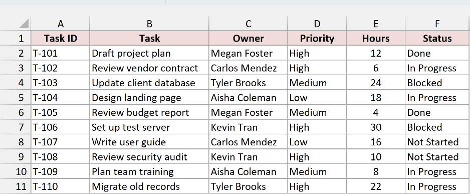
Below I have the same task list, and I want to highlight the tasks that are Not Started.

Here are the steps to do this:

1. Select any cell in the data and press Ctrl + Shift + L (Cmd + Shift + F on a Mac) to add filter buttons to the headers.
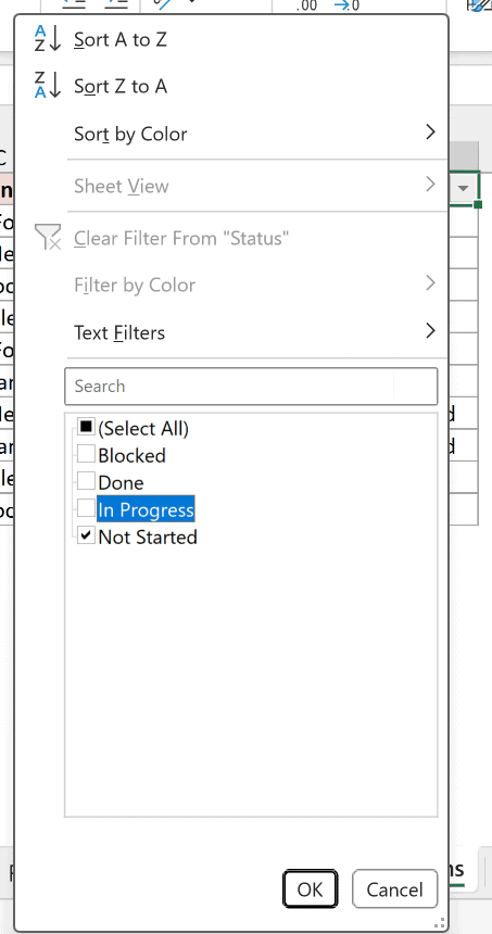
2. Click the filter arrow in the Status header, uncheck (Select All), check Not Started, and click OK.

3. Select the visible data rows (A8:F9 here), without the header.

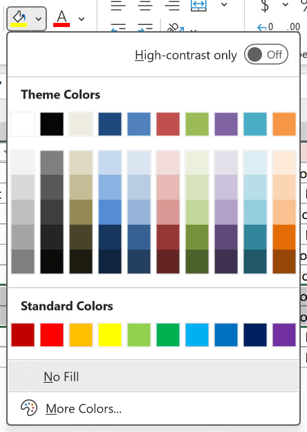
4. On the Home tab, click the Fill Color drop-down and pick a light color.

5. Press Ctrl + Shift + L again to remove the filter.

All the rows are back, and only the two Not Started tasks, T-107 and T-108, keep the fill.

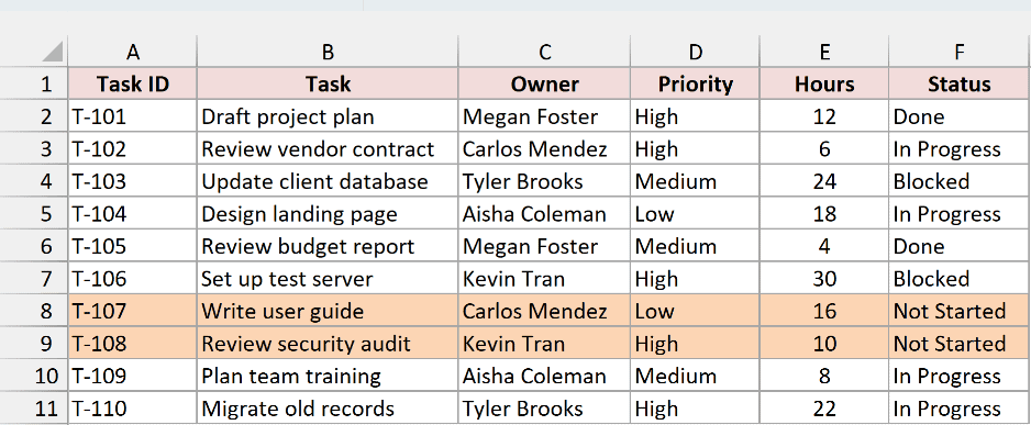
When the data is filtered, Excel formats only the visible rows.

So if your matching rows are spread out, you can select them all at once and the hidden rows stay uncolored.

Additional Notes About Highlighting Rows Based on Cell Value in Excel

• New rows can miss the rule. A rule applied to A2:F11 stops at row 11. Convert the data to an Excel Table (Ctrl + T), and the rule grows with the table as you add rows below it.
• Text checks ignore case. Both = and SEARCH treat “blocked” and “Blocked” the same. If case matters, use FIND instead of SEARCH, since FIND is case-sensitive.
• Conditional formatting sits on top of manual fill. If a row already has a fill color, the rule’s color shows while the rule is TRUE. Your manual color comes back when it isn’t.
• The example file has every rule in place. Open Manage Rules on any sheet to see the exact formula and range behind it.

Frequently Asked Questions

Here are some common questions people ask about highlighting rows based on a cell value.

Can I highlight a row based on a date in Excel?

Yes. Use a date comparison in the formula rule. For example, if column C has due dates, =$C2<TODAY() highlights every row whose due date has already passed.

Will the highlight update when the cell value changes?

Yes, for Methods 1 through 5. Conditional formatting rechecks the rule whenever the data changes. Only the filter-and-fill method gives a fixed color that won’t update.

How do I highlight a column instead of a row based on a cell value?

Flip the dollar sign so it locks the row instead of the column.

For example, select B2:M11 and use =B$1=”Mar” to highlight the column whose header in row 1 says Mar.

How do I remove the row highlighting?

Select the range, then go to Home > Conditional Formatting > Clear Rules > Clear Rules from Selected Cells. To delete just one rule, use Manage Rules instead.

Conclusion

In this article, I showed you six ways to highlight a row based on a cell value in Excel.

They range from a basic formula rule to SEARCH, AND, color rules, a drop-down, and filter and fill.

For most cases, the formula rule with the column locked, like =$F2=”Blocked”, is the one to reach for.

I hope you found this article helpful.

Other Excel articles you may also like:

• Highlight Cell If Value Exists in Another Column in Excel
• Change Cell Color Based on Value of Another Cell in Excel
• Change Cell Color Based on Text Input in Excel
• How to Highlight Duplicates in Excel
• How to Highlight Every Other Row in Excel (Conditional Formatting & VBA)
• How To Highlight Weekends In Excel?
• How to Change Font Color Based on Cell Value in Excel?
• How to Highlight Blank Cells in Excel?