How to Highlight Duplicates in Excel

If you want to spot the repeated entries in an Excel sheet, coloring them in is the fastest way to see what you’re dealing with. But Excel’s built-in rule compares one cell to another, so it never tells you a whole record is repeated.

That’s easy enough to fix once you know which rule to reach for. In this article I’ll show you six ways to highlight duplicates in Excel, starting with the two-click option and finishing with a macro.

Everything here is about coloring duplicates, not getting rid of them. If you’d rather filter them out or delete them than color them, our guide on how to find duplicates in Excel covers that side.

Method #1: Use the Duplicate Values Rule to Highlight Duplicates in Excel

Excel has a duplicate highlighter built into Conditional Formatting, and for most jobs it’s all you need. Reach for this one when you have a single column of names, emails, or IDs and you just want to see what repeats.

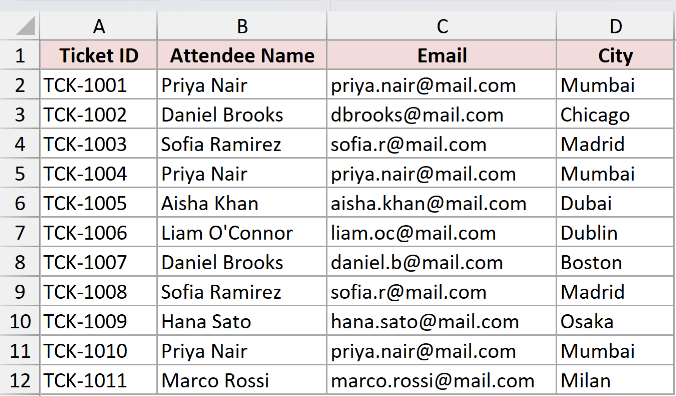
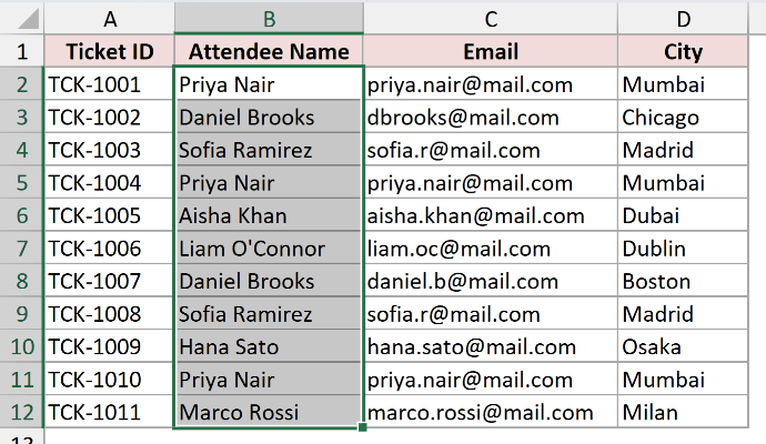
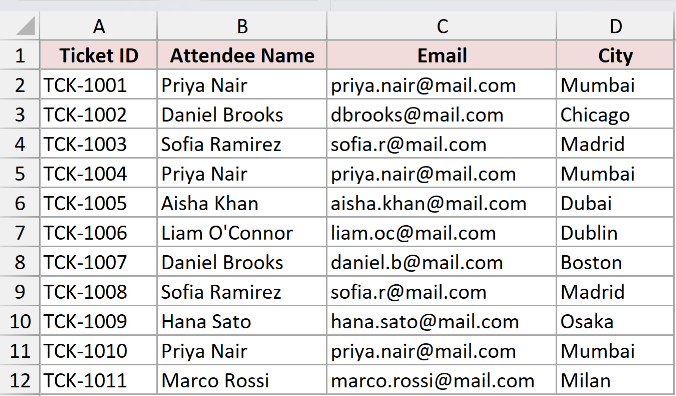
Below I have a workshop registration list on a sheet called Registrations. It has the ticket ID, attendee name, email, and city in A1:D12, and I want to see which attendee names show up more than once.

Here are the steps to highlight duplicates using the Duplicate Values rule:

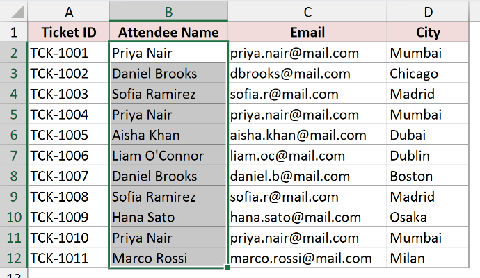
1. Select the range that has the names (B2:B12).

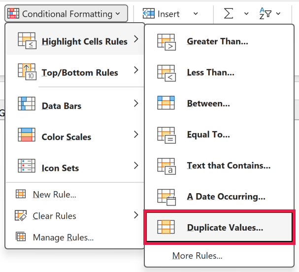
2. On the Home tab, click Conditional Formatting, then Highlight Cells Rules, then Duplicate Values.

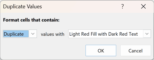
3. In the Duplicate Values dialog box, leave the first drop down set to Duplicate and pick a format from the second drop down.

4. Click OK.

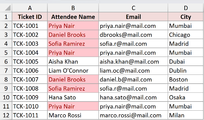
Priya Nair, Daniel Brooks, and Sofia Ramirez all light up. The four one-off names stay plain. Two clicks, no formula, and nothing you can anchor incorrectly.

There is one thing this rule cannot do, though, and it’s the reason the next method exists. The Duplicate Values rule works cell by cell.

Select all four columns (A2:D12), apply it, and Excel doesn’t compare rows at all. It colors any value that repeats anywhere inside the block, so Mumbai and Madrid get painted right alongside the names.

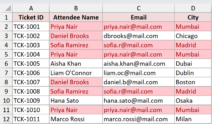
Nothing about a repeated city makes a registration a duplicate. You end up with a patchwork of colored cells instead of an answer, which is why the built-in rule belongs on one column at a time.

Method #2: Use a COUNTIF Formula Rule to Highlight Duplicate Rows in Excel

Here’s the step up from Method #1, and it’s the one to move to the moment your data is a table of records rather than a list.

Instead of letting Excel decide what a duplicate is, you write your own rule that counts one key column and colors the whole row when that name repeats.

Same registration list on the Registrations sheet, with the ticket ID, attendee name, email, and city in A1:D12. This time I want the entire row to color when the attendee name shows up more than once.

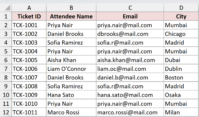
Note: “Duplicate row” here means a repeated name, email, and city, not a literally identical row. The Ticket ID never repeats, because the system issues a fresh ID for every signup, so it can never be part of the test.

Here is the formula:

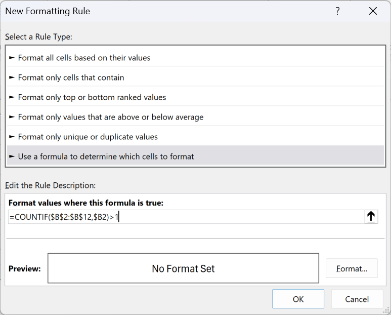
=COUNTIF($B$2:$B$12,$B2)>1

How does this formula work?

The COUNTIF function counts how many times a value appears in a range. Here it counts how many times the name in B2 shows up across the whole name column, B2:B12.

If the count comes back greater than 1, the formula returns TRUE and Excel paints the cell. Otherwise it returns FALSE and the cell is left alone.

The dollar signs are doing the real work. $B$2:$B$12 is locked completely, so every cell in the table tests against the same list of names.

$B2 locks the column but not the row. Column B is locked so all four cells in a row check the same name, and the row is free so the rule walks down the table as it goes.

Select the range the right way before you open the dialog box. This part gets skipped constantly, and it is the number one reason these rules “don’t work”.

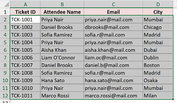
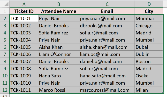
A formula rule is written from the point of view of the active cell, which is the single white cell inside the highlighted block. Drag from A2 down to D12 so that A2 stays active.

Drag bottom-up from D12 instead and A12 becomes active. Excel then anchors the rule to row 12, and your highlighting lands ten rows away from where you wanted it.

Here are the steps to highlight duplicate rows with a COUNTIF rule:

1. Select A2:D12, starting at A2 and dragging down, so that A2 is the active cell.

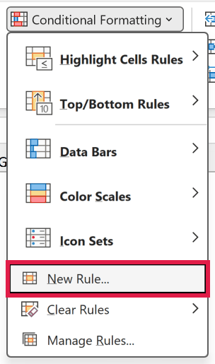
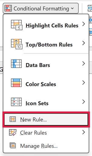
2. On the Home tab, click Conditional Formatting, then New Rule.

3. In the New Formatting Rule dialog box, select “Use a formula to determine which cells to format” and enter the formula above in the box below it.

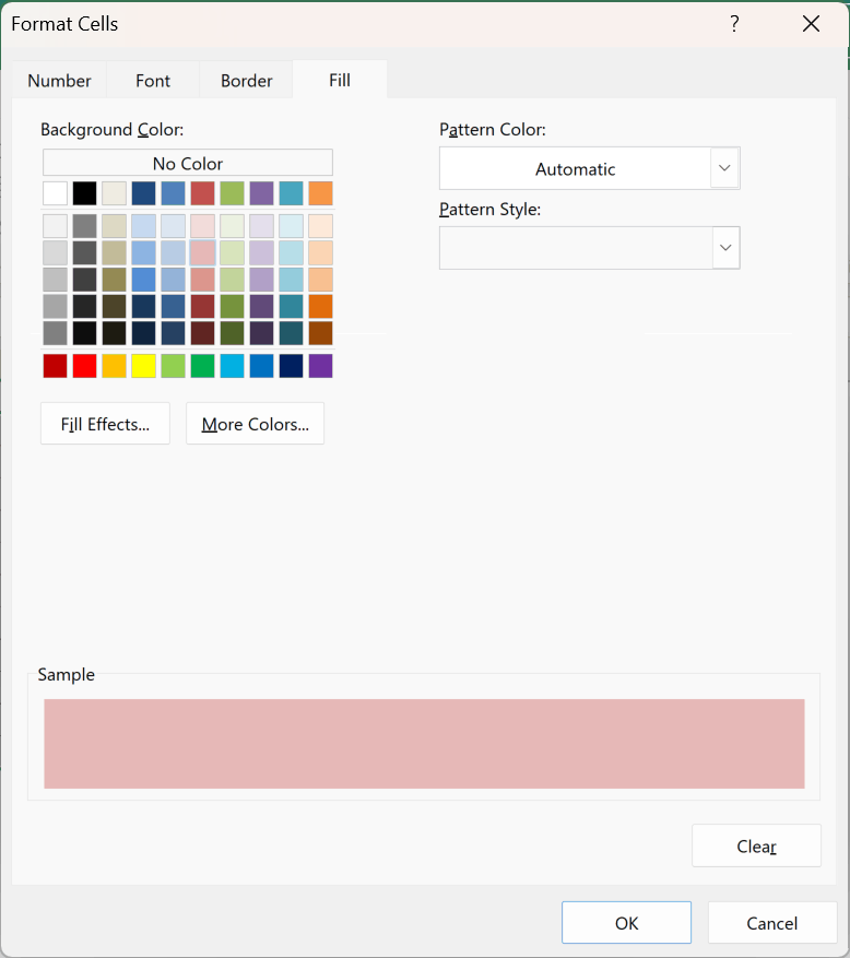
4. Click the Format button, go to the Fill tab, pick a color, and click OK.

5. Click OK to apply the rule.

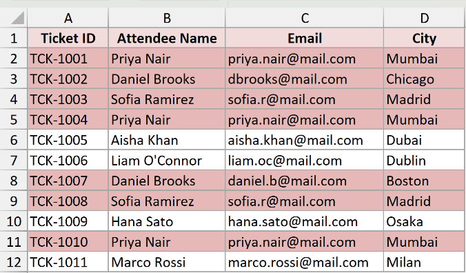
The rows for Priya Nair, Daniel Brooks, and Sofia Ramirez are now colored end to end, ticket ID through city. The cities no longer color on their own, because the rule only ever looks at column B.

Method #3: Apply the COUNTIFS Function to Highlight Duplicates Across Multiple Columns in Excel

Method #2 trusts one column. That’s fine when names are genuinely unique, but two different people can share a name, and then you’re coloring a row that isn’t a duplicate at all.

This method checks every column before it calls anything a match. Use it when the data has to agree on more than one field to count as a repeat.

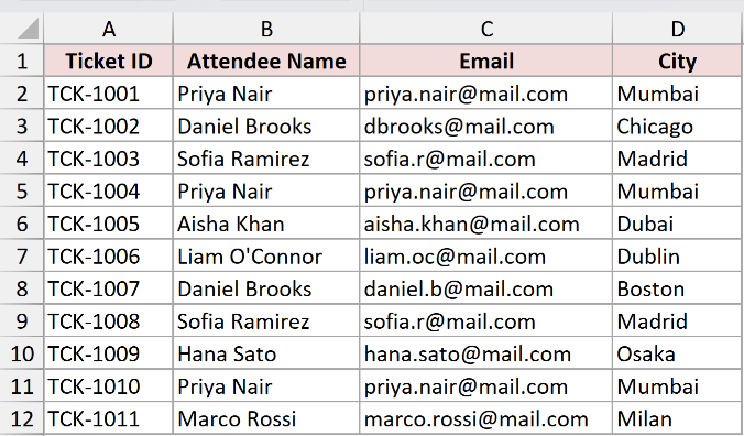
Same registration list on Registrations, with the ticket ID, attendee name, email, and city in A1:D12. This time a row only counts as a duplicate when the name, the email, and the city all match another row.

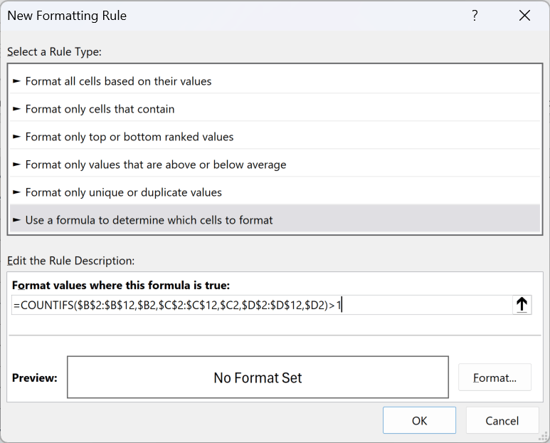
Here is the formula:

=COUNTIFS($B$2:$B$12,$B2,$C$2:$C$12,$C2,$D$2:$D$12,$D2)>1

How does this formula work?

The COUNTIFS function is COUNTIF with more than one condition. It only counts a row when every condition is true at the same time.

The three pairs check the name against the name column, the email against the email column, and the city against the city column.

The anchoring follows the exact same pattern as Method #2. Each range is locked completely, and each criteria reference is the $B2 shape, column locked and row free.

If the count is greater than 1, that combination of name, email, and city exists somewhere else in the list, so it’s a real repeat.

Here are the steps to highlight duplicates across multiple columns:

1. Select A2:D12, starting at A2 and dragging down, so that A2 is the active cell.

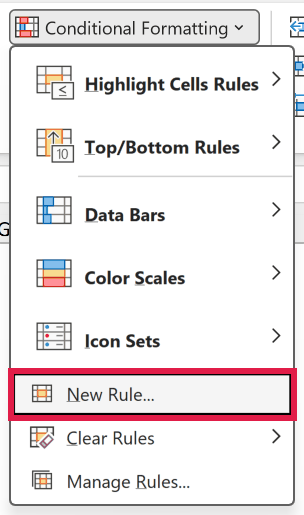
2. On the Home tab, click Conditional Formatting, then New Rule.

3. In the New Formatting Rule dialog box, select “Use a formula to determine which cells to format” and enter the formula above in the box below it.

4. Click the Format button, pick a fill color on the Fill tab, then click OK twice to apply the rule.

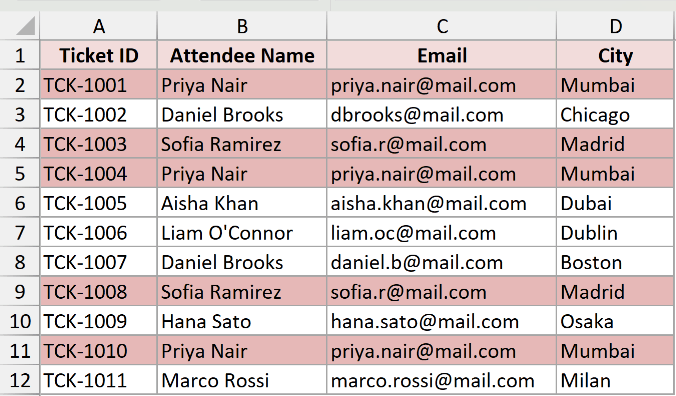
Now look at what changed. Priya Nair’s three rows are still colored, and so are Sofia Ramirez’s two. Daniel Brooks is not.

His two rows share a name, but row 3 is dbrooks@mail.com in Chicago and row 8 is daniel.b@mail.com in Boston. They’re two different people who happen to be called Daniel Brooks.

Method #1 and Method #2 both colored him. This rule leaves him alone, and that’s the whole reason to check every column instead of just one.

Note: COUNTIFS accepts up to 127 range and criteria pairs, so you can keep adding columns well past anything a normal table needs. Every range you add has to be the same size as the others.

Method #4: Use an Expanding COUNTIF Range to Highlight Duplicates Except the First Occurrence in Excel

Sometimes the first entry isn’t the problem. The repeats are. If you want to keep the original clean and see only the extras, the rule has to look backwards rather than at the whole column.

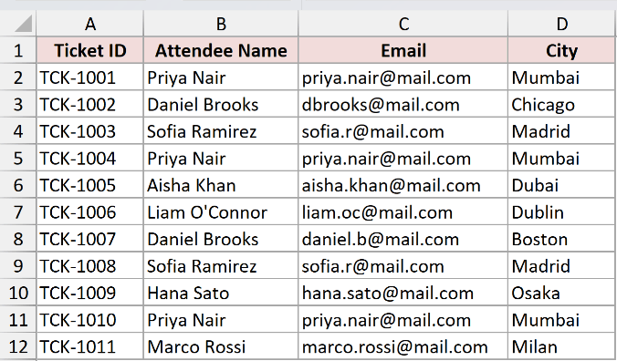
Same Registrations list, with the ticket ID, attendee name, email, and city in A1:D12. This time I only want the second and third time a name appears to color, leaving the first one plain.

Here is the formula:

=COUNTIF($B$2:$B2,$B2)>1

How does this formula work?

Look closely at the range. It’s $B$2:$B2, not $B$2:$B$12. The start is locked and the end is not, so the range grows as the rule moves down the column.

In B2 the range is only B2, so the count is 1 and nothing colors. Down at B5 the range has stretched to B2:B5, and Priya Nair has now appeared twice, so that one colors.

By B11 the range is B2:B11 and Priya is on her third appearance, so it colors as well.

Every value’s first appearance always counts 1, because there’s nothing above it to match against. Anything after that counts 2 or more and gets painted.

That half-locked range is the entire trick. Write $B$2:$B$12 by mistake and you’re straight back to Method #2, with every occurrence colored.

Here are the steps to highlight duplicates except the first occurrence:

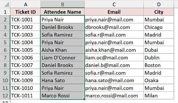
1. Select B2:B12, starting at B2 and dragging down, so that B2 is the active cell.

2. On the Home tab, click Conditional Formatting, then New Rule.

3. In the New Formatting Rule dialog box, select “Use a formula to determine which cells to format” and enter the formula above in the box below it.

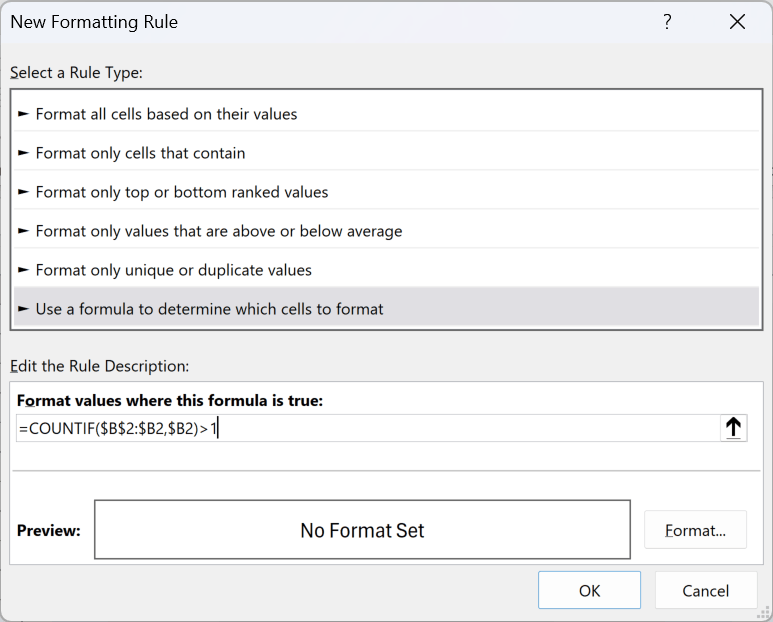
4. Click the Format button, pick a fill color on the Fill tab, then click OK twice to apply the rule.

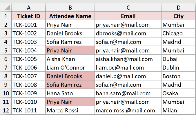
Four cells color: B5, B8, B9, and B11. That’s Priya Nair’s second and third entries, Daniel Brooks’s second, and Sofia Ramirez’s second. The first of each stays plain.

Note: Because the rule reads from the top down, “first occurrence” means first in the order the list is sitting in right now. Sort the list differently and a different row keeps the clean fill.

Method #5: Use a COUNTIF Rule to Highlight Duplicates in Two Sheets in Excel (Excel 2010 Onwards)

Here’s another one, for when the list you’re comparing against lives somewhere else in the workbook. You can point a COUNTIF rule at a second sheet and color everyone who shows up on both.

If both lists are sitting side by side on the same sheet instead, our guide on how to highlight a cell if the value exists in another column covers that setup. This method is the two-sheet version.

Below I have the same Registrations list, with the ticket ID, attendee name, email, and city in A1:D12.

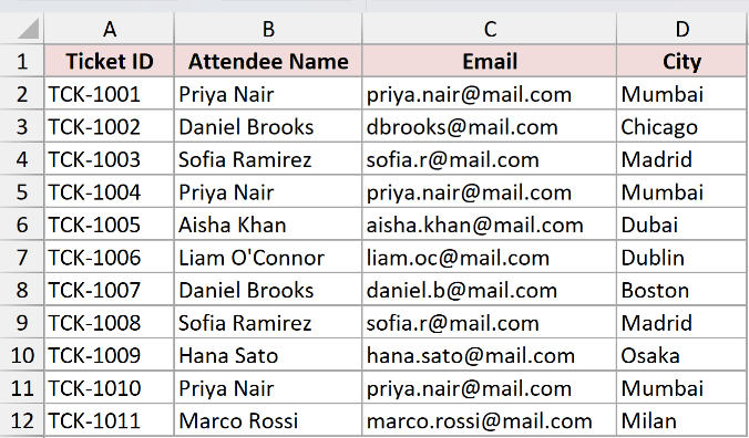
And here is a second sheet called Last Year, holding a shorter list of the people who came to the previous workshop. It has the ticket ID in column A and the attendee name in column B.

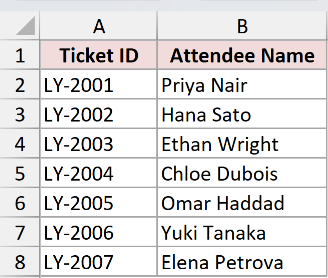
I want to color the names on Registrations that also appear on Last Year, so the returning attendees stand out.

Here is the formula:

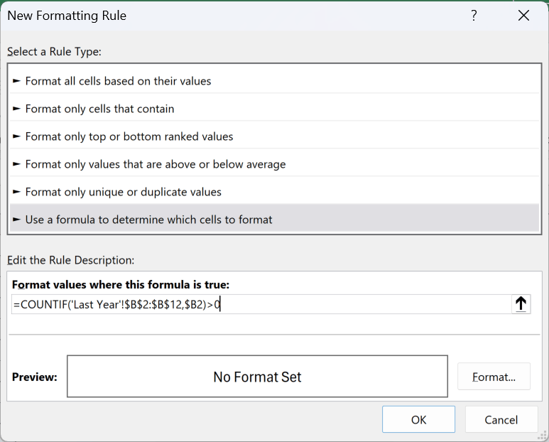
=COUNTIF('Last Year'!$B$2:$B$12,$B2)>0

How does this formula work?

The range now points at column B of the Last Year sheet. The sheet name sits in single quotes because it has a space in it, and Excel adds those for you when you click the range.

Notice the >0. This is the part people get wrong.

In the earlier methods you were counting a column against itself, so every name found itself once and you needed a count above 1 to prove a repeat.

Here you are counting against a completely different list, so a name isn’t in there by default. One single hit already means that person attended both years.

Writing >1 here fails quietly. You would only color people who registered twice last year, and everyone else would look clean even when they’re not.

The range runs down to row 12 even though Last Year only holds seven names. That’s harmless, because a blank cell never matches a name, and it leaves room for the list to grow.

Here are the steps to highlight duplicates in two sheets:

1. On the Registrations sheet, select B2:B12, starting at B2 and dragging down, so that B2 is the active cell.

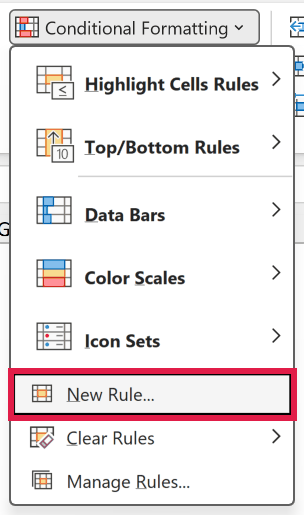
2. On the Home tab, click Conditional Formatting, then New Rule.

3. In the New Formatting Rule dialog box, select “Use a formula to determine which cells to format” and enter the formula above in the box below it.

4. Click the Format button, pick a fill color on the Fill tab, then click OK twice to apply the rule.

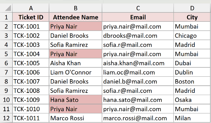
Priya Nair and Hana Sato color. All three of Priya’s name cells light up, since every one of them carries a name that’s on last year’s list.

Note: Pointing a conditional formatting formula straight at another sheet needs Excel 2010 or later. In Excel 2007 and earlier the rule will not accept it, and the workaround is to create a named range for the other sheet’s list and use that name in the formula instead.

Method #6: Run a VBA Macro to Highlight Duplicates in Excel

If you do this on the same report every week, a macro turns the whole job into one click. It’s also what you want when the colors need to stay put rather than react to the data.

Same Registrations list, with the ticket ID, attendee name, email, and city in A1:D12, and the goal is to color the attendee names that repeat.

Here is the VBA code:

Sub HighlightDuplicateNames()
    Dim rng As Range
    Dim cel As Range

    Set rng = ThisWorkbook.Worksheets("Registrations").Range("B2:B12")
    rng.Interior.ColorIndex = xlNone

    For Each cel In rng
        If cel.Value <> "" Then
            If Application.WorksheetFunction.CountIf(rng, cel.Value) > 1 Then
                cel.Interior.Color = RGB(255, 199, 206)
            End If
        End If
    Next cel
End Sub

Sub HighlightDuplicateNames()
    Dim rng As Range
    Dim cel As Range

    Set rng = ThisWorkbook.Worksheets("Registrations").Range("B2:B12")
    rng.Interior.ColorIndex = xlNone

    For Each cel In rng
        If cel.Value <> "" Then
            If Application.WorksheetFunction.CountIf(rng, cel.Value) > 1 Then
                cel.Interior.Color = RGB(255, 199, 206)
            End If
        End If
    Next cel
End Sub

Here are the steps to use this macro:

1. Press Alt + F11 to open the VBA Editor
2. Insert a new module (Insert → Module)
3. Paste the code above
4. Press F5 to run the macro

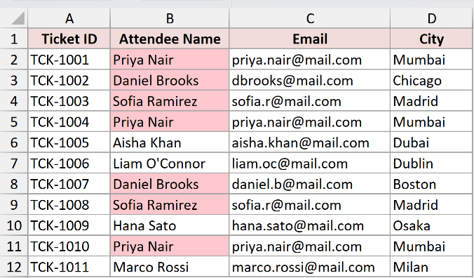
The macro grabs B2:B12 on the Registrations sheet and clears any fill that’s already sitting there, so a second run never leaves old colors behind.

Then it walks the cells one at a time. For each one it runs the same COUNTIF you saw in Method #2, and if the count comes back above 1 it paints that cell light red.

The cel.Value <> "" check keeps empty cells out of it. Without that line, every blank in the range would match every other blank and get colored.

Note: This fill is static. Unlike conditional formatting, it will not update when you edit the data, so you have to run the macro again. You also need to save the workbook as a macro-enabled file (.xlsm) if you want to keep the code.

Additional Notes About Highlighting Duplicates in Excel

• Trailing spaces defeat every method here. Priya Nair with a space on the end simply isn’t the same value as Priya Nair, and nothing will color. Run the column through the TRIM function before you build the rule, especially with pasted or exported data.
• COUNTIF converts text that looks like a number, so an ID of 07023 and one of 7023 count as the same value. IDs longer than 15 digits only compare on their first 15 digits. When your IDs are stored as text, add &"*" to the criteria to force a text comparison: =COUNTIF($B$2:$B$12,$B2&"*")>1.
• Blank cells count as duplicates of each other. Any empty cell inside the range matches every other empty cell and colors, which is rarely what you want unless you set out to highlight blank cells on purpose. Wrap the rule to skip them with =AND($B2<>"",COUNTIF($B$2:$B$12,$B2)>1).
• Power Query can’t color anything. It applies no cell formatting at all, so the best it can do is group your list and hand you a count column, and you’d still need a conditional formatting rule on that count to see the repeats. If getting rid of them is the goal rather than seeing them, Power Query’s Remove Duplicates is the right tool.
• Coloring isn’t the only way to read repeats. If you’d rather pull the repeated entries next to each other so you can count or total them, group duplicates in Excel does that with a rule plus a sort.

Frequently Asked Questions

Why is Excel highlighting values that aren’t actually duplicates?

Almost always because the built-in Duplicate Values rule works cell by cell rather than row by row. Point it at more than one column and it colors any value repeating anywhere in the block, so a city lights up on its own.

Use Method #2 or Method #3 instead. Both of those test the row rather than the individual cell.

If the flagged values genuinely look identical to you, check for a trailing space or a number stored as text. Both change what Excel counts as a match.

Can Excel highlight duplicates case-sensitively?

Not with COUNTIF or with the built-in rule. Both treat priya nair and Priya Nair as the same value.

For a case-sensitive rule, use EXACT inside SUMPRODUCT instead:

=SUMPRODUCT(--EXACT($B$2:$B$12,$B2))>1

EXACT compares every name in the range against B2 and respects capitalization. The double minus turns the TRUEs into 1s so that SUMPRODUCT can add them up.

How do I change the duplicate highlight to a different color?

Go to the Home tab, click Conditional Formatting, then Manage Rules. Set the drop down at the top to “This Worksheet”, pick your rule, and click Edit Rule.

Click the Format button, choose a new fill on the Fill tab, then click OK on your way back out. The existing highlighting recolors straight away.

Why does my duplicate highlighting stop working when I add new rows?

A conditional formatting rule only covers its Applies to range. Type a row below that range and it falls outside the rule, so nothing colors.

Convert your data to an Excel Table with Ctrl + T before you create the rule. A Table extends its conditional formatting to new rows on its own, so the Applies to range keeps up.

The range inside the formula needs the same treatment. Swap $B$2:$B$12 for the whole column, $B:$B, and it will never run short.

How do I remove the duplicate highlighting when I’m done?

Select the range, then go to the Home tab, click Conditional Formatting, then Clear Rules, then Clear Rules from Selected Cells. To wipe every rule on the sheet at once, pick Clear Rules from Entire Sheet instead.

If you used the macro from Method #6, Clear Rules will not touch it, because that’s a real fill rather than a rule. Select the cells and set the fill back to No Fill from the Home tab.

Conclusion

We covered six ways to highlight duplicates in Excel: the built-in Duplicate Values rule, COUNTIF and COUNTIFS rules that color a whole row, an expanding range for the repeats only, a cross-sheet rule, and a VBA macro.

For a single column of names or emails, start with Method #1. The moment your data is a table of records rather than a list, move to Method #2 or #3, and select from the top down so the rule anchors where you expect.

Other Excel articles you may also like:

• How to Remove Duplicate Rows based on one Column in Excel?
• How to Highlight Every Other Row in Excel (Conditional Formatting & VBA)
• How to Compare Two Columns in Excel (using VLOOKUP & IF)
• Using Conditional Formatting with OR Criteria in Excel
• Highlight Cells with Formulas in Excel
• MOD Function in Excel
• Change Cell Color Based on Value of Another Cell in Excel
• How to Check If a Cell Contains Text in Excel?