
The SUMIFS function in Excel adds up values that meet every condition you give it. That’s AND logic, so the moment you want sales for Denver OR Austin, a plain SUMIFS formula can’t do it.
Arrays fix that. When you hand SUMIFS a list of criteria instead of one value, it calculates a separate total for each item in the list, and you add those totals up.
The catch is that SUMIFS only takes arrays in some of its arguments. Its sum range and criteria ranges have to be real cell ranges, so a calculated array, like month numbers worked out from a date column, won’t work there.
In this article, I’ll show you how to use array constants and cell ranges as criteria, combine two arrays into a grid of totals, point SUMIFS at a spilled helper column, and switch to SUMPRODUCT when SUMIFS won’t take the array.
Which SUMIFS Arguments Accept Arrays
Before the methods, it helps to know where an array can go. SUMIFS has three kinds of arguments, and they don’t all treat arrays the same way.
| Argument | Array constant like {"Denver","Austin"} | Cell range or spill reference like G2:G4 or F2# | Calculated array like MONTH(B2:B13) |
|---|---|---|---|
| sum_range | No | Yes | No |
| criteria_range | No | Yes | No |
| criteria | Yes | Yes | Yes |
So arrays belong in the criteria argument. The two range arguments need cells that actually exist on a sheet. A spill reference counts, because it points to real cells.
If you type something like =SUMIFS(E2:E13,MONTH(B2:B13),1), Excel won’t accept the formula at all. It shows an error message instead of a result. Methods #4 and #5 show you two ways around that.
Method #1: Using an Array Constant as the Criteria
This is the method I’d reach for first. You type the items you want right inside the formula, between curly braces, and SUMIFS does the rest.
Below I have a dataset of coffee orders with the order date, city, roast, and sales amount. I want the total sales for Denver and Austin combined.
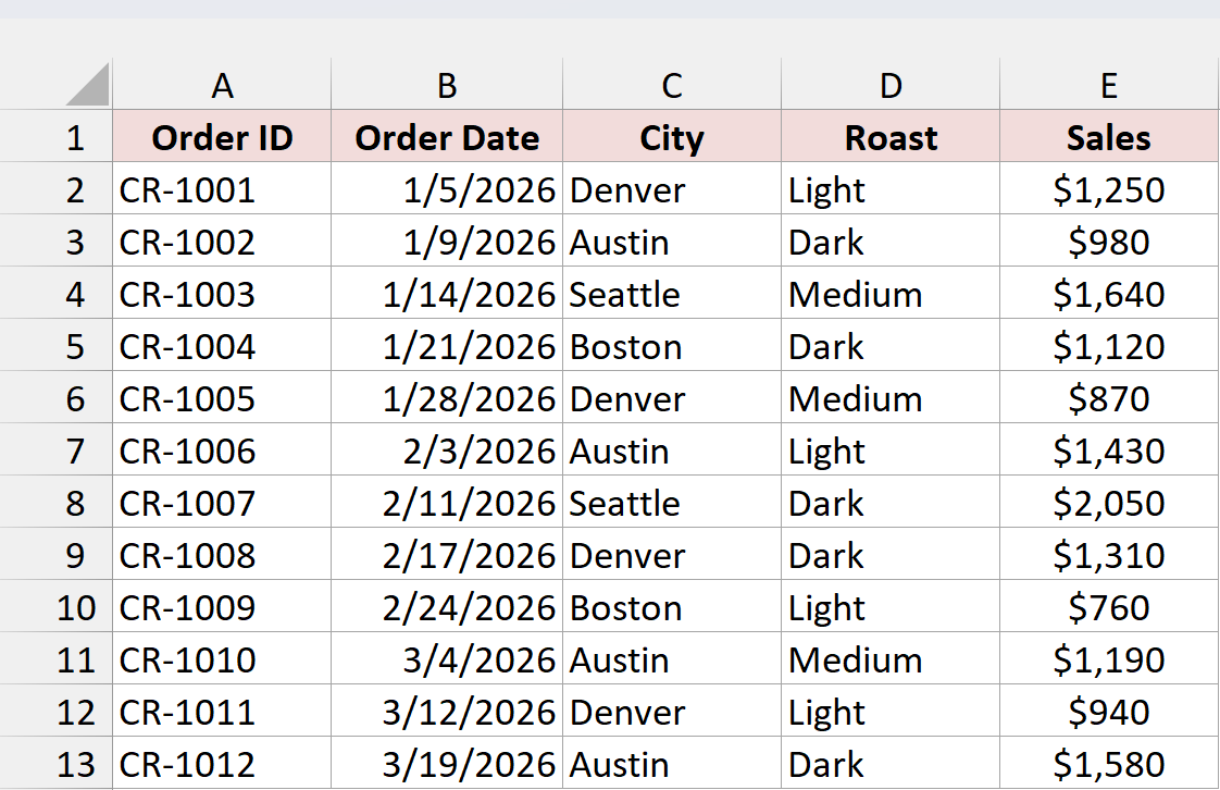
First, let’s see what SUMIFS does with a list of cities. I entered this formula in G2:
=SUMIFS(E2:E13,C2:C13,{"Denver","Austin"})
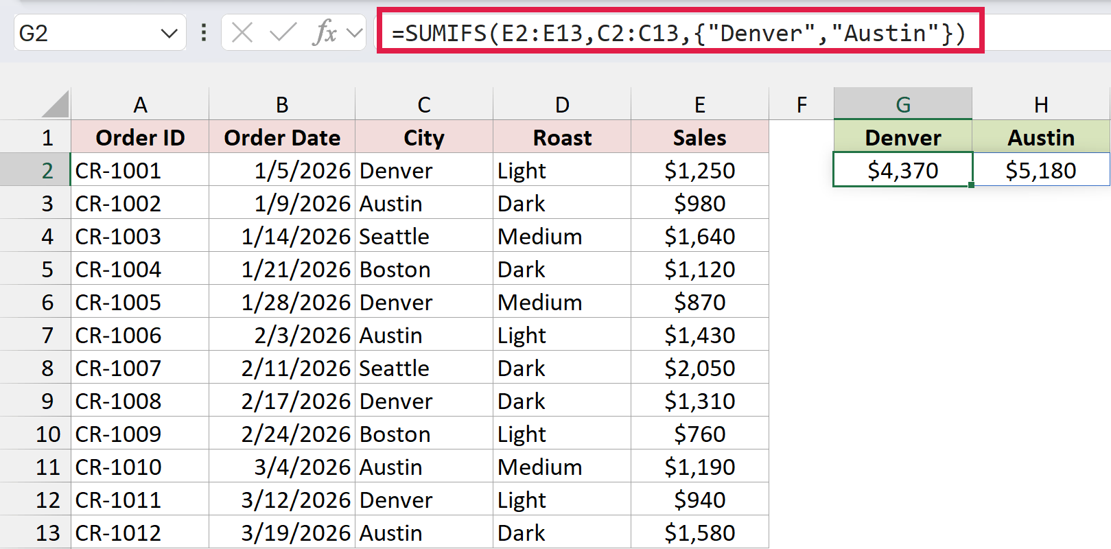
You get two results that spill across G2:H2. $4,370 is the Denver total and $5,180 is the Austin total.
To turn those two numbers into one total, wrap the formula in SUM. Here is the formula I used in J2:
=SUM(SUMIFS(E2:E13,C2:C13,{"Denver","Austin"}))
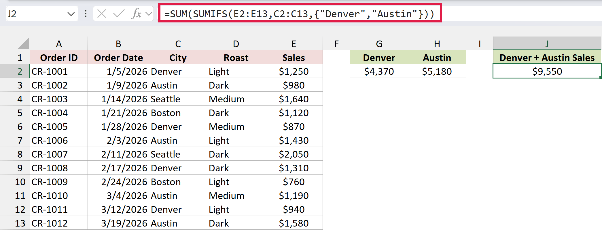
This returns $9,550, the combined sales for both cities.
How does this formula work?
The part in curly braces, {"Denver","Austin"}, is an array constant. It’s a fixed list of values typed straight into the formula.
When SUMIFS gets an array in its criteria argument, it runs once for each item. It sums column E where column C is Denver, then again where column C is Austin. That gives you the two totals you saw in G2:H2.
SUM then adds those totals together. Because each row can only match one city, nothing gets counted twice, and you end up with an OR result: sales for Denver or Austin.
Note: The SUM version works in older versions of Excel too, and you don’t need Ctrl + Shift + Enter, because the criteria come from an array constant. The spill of separate totals in G2:H2 needs Excel 2021 or newer (including Microsoft 365).
Method #2: Using a Cell Range as the Criteria
Typing the items into the formula is fine for two or three values. When the list is longer, or it changes often, keep the criteria in cells and point SUMIFS at them instead.
Below I have the same coffee orders, plus a list of the cities I want in G2:G4 (Denver, Seattle, and Boston).
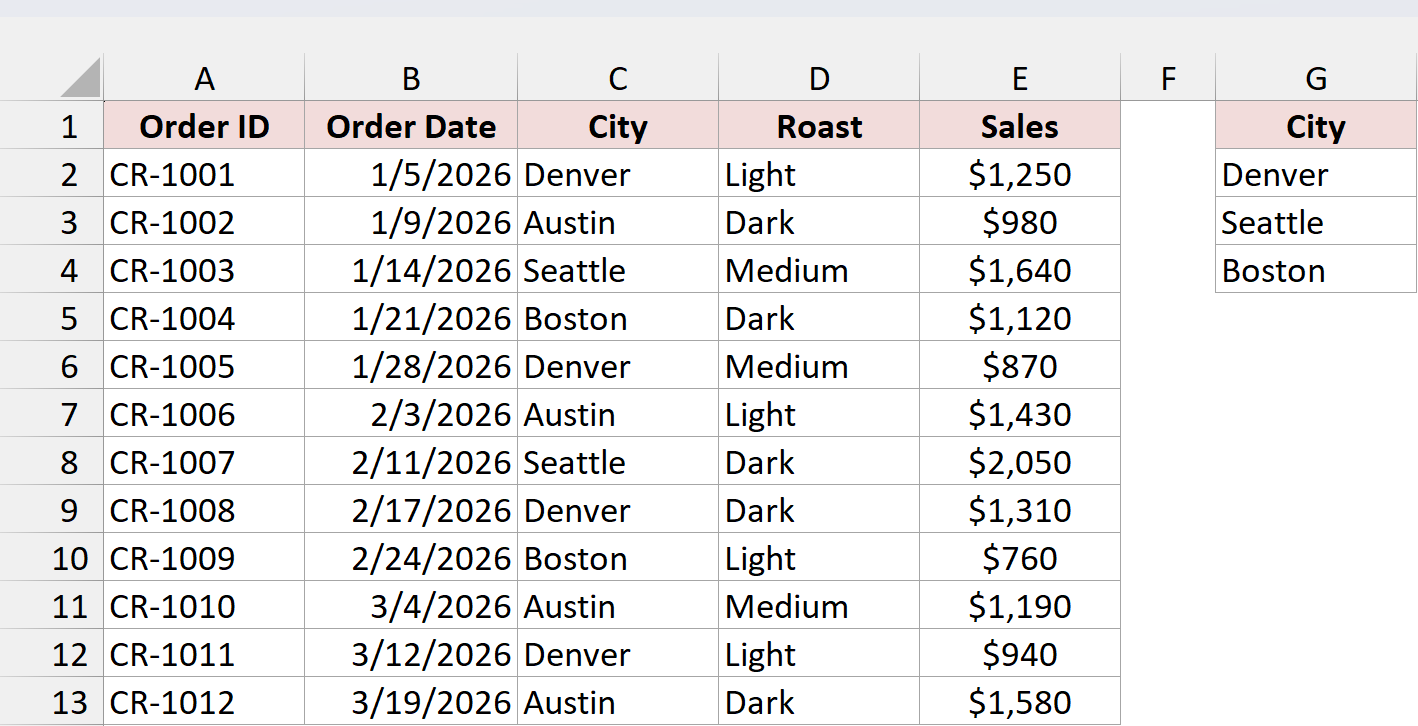
Here is the formula I entered in H2:
=SUMIFS(E2:E13,C2:C13,G2:G4)
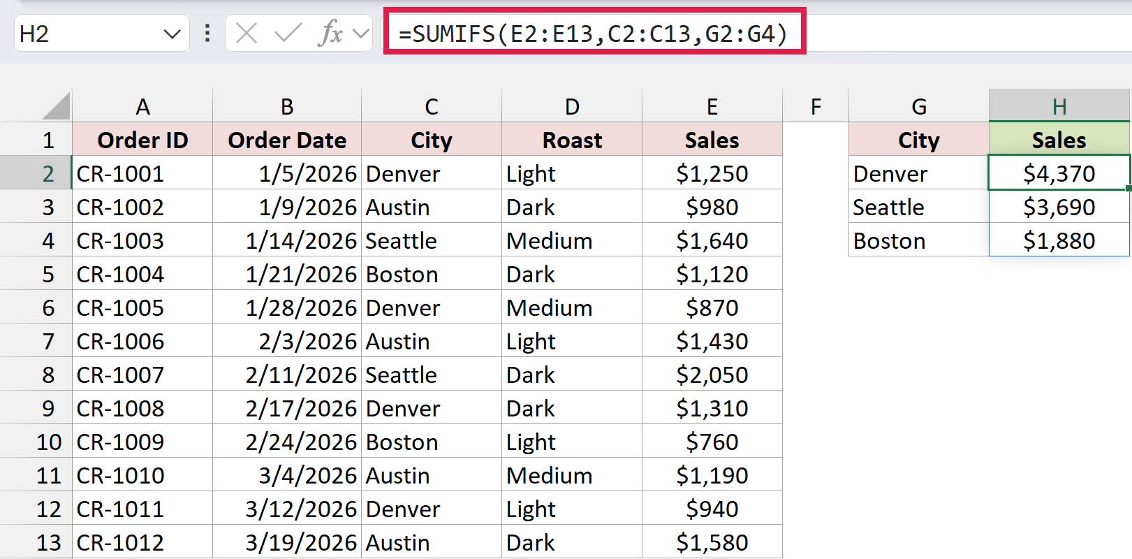
The formula spills down H2:H4 and returns a total for each city in the list: $4,370 for Denver, $3,690 for Seattle, and $1,880 for Boston.
If you just want one number for all three cities, wrap the same formula in SUM. I entered this one in H5:
=SUM(SUMIFS(E2:E13,C2:C13,G2:G4))
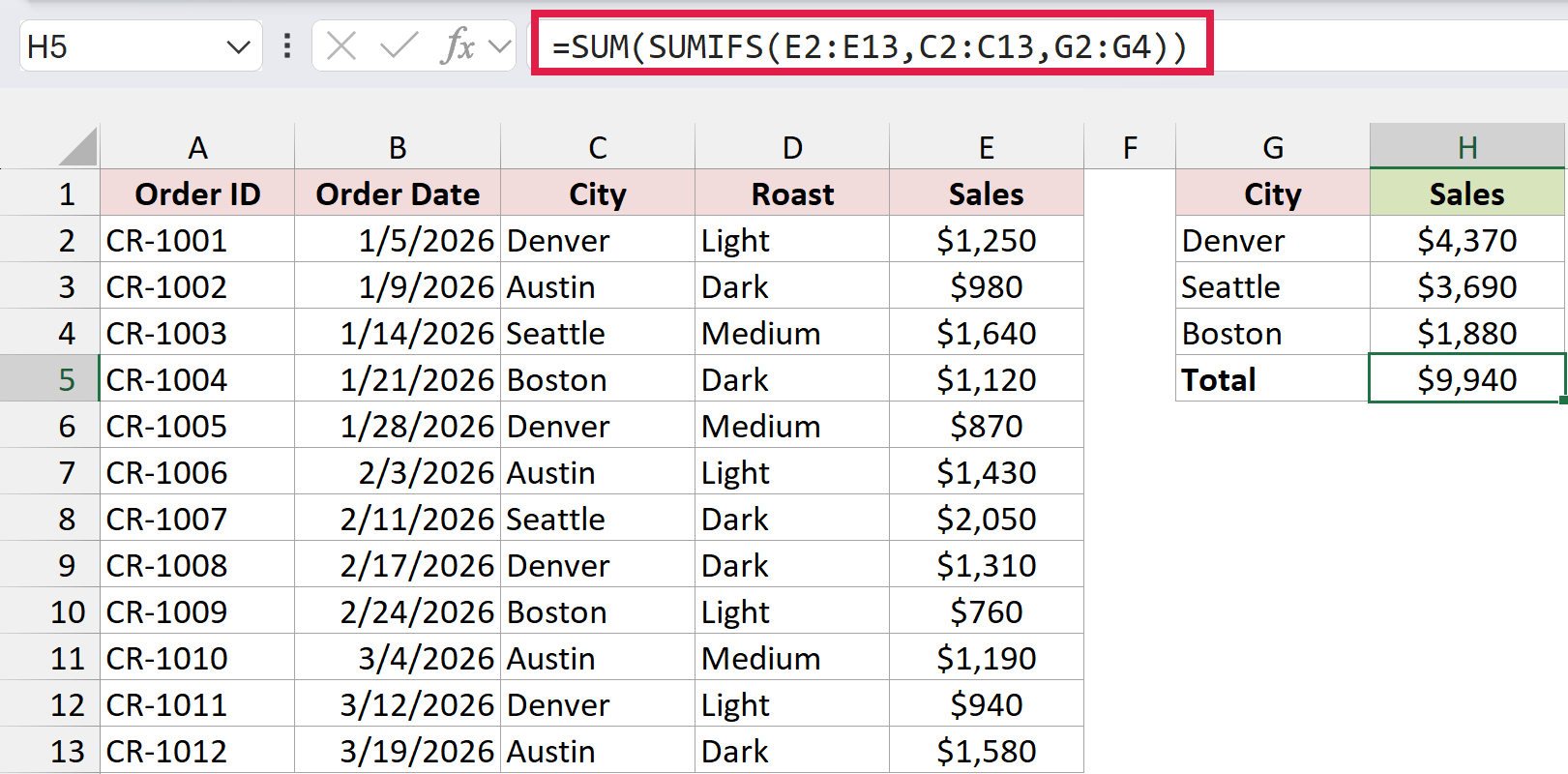
This returns $9,940, which is the three city totals added together.
How does this formula work?
G2:G4 works just like the array constant in Method #1. SUMIFS takes each city in that range, one at a time, and returns a separate total for each one.
Without SUM, Excel shows those totals as a spilled list next to your criteria. With SUM, they get added into one grand total.
The nice part is that you can change the cities in G2:G4 and both formulas update right away. You never have to edit the formula itself.
Note: In Excel 2019 and earlier, the SUM version with a cell range needs to be entered with Ctrl + Shift + Enter. If you press Enter only, older Excel doesn’t evaluate the whole list, and you get the wrong total.
Method #3: Using Two Arrays in Different Orientations
You can also give SUMIFS one list for the city and another list for the roast, and get every combination in one formula.
The trick is the separator. A comma inside the braces puts items side by side in a row. A semicolon stacks them in a column.
Below I have the coffee orders again. I want the sales where the city is Denver or Austin AND the roast is Light or Dark.
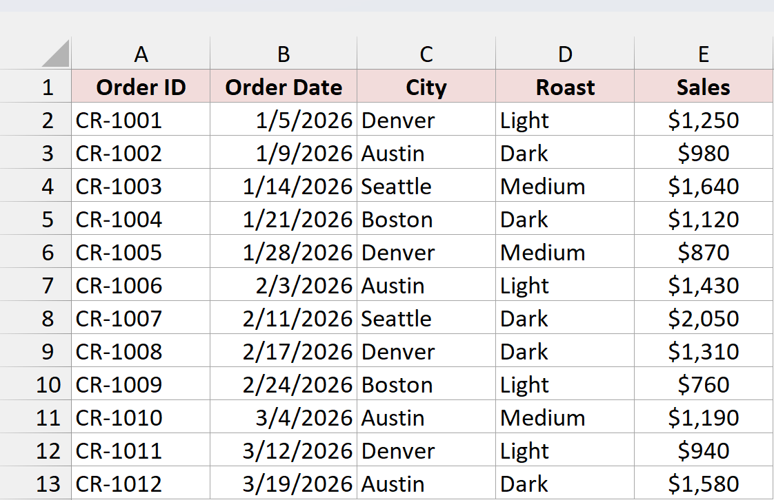
Here is the formula I entered in H2:
=SUMIFS(E2:E13,C2:C13,{"Denver","Austin"},D2:D13,{"Light";"Dark"})
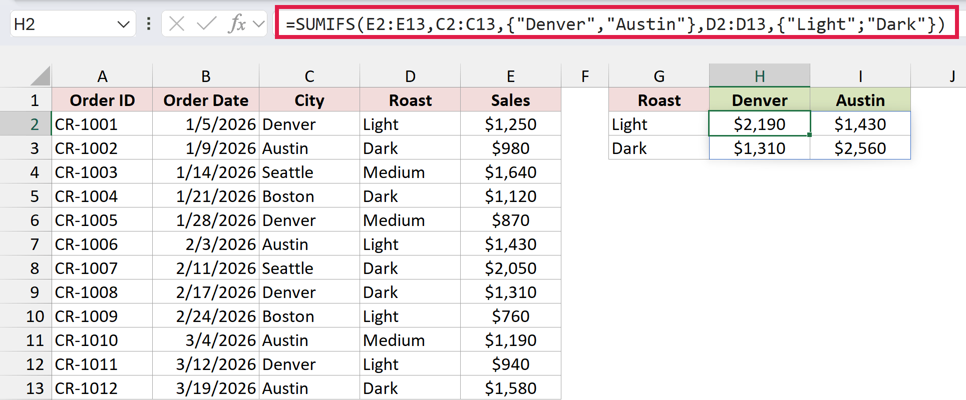
The cities go across (comma) and the roasts go down (semicolon), so the formula spills a 2-by-2 grid into H2:I3. For example, H2 is Denver Light ($2,190) and I3 is Austin Dark ($2,560).
To get one total for all four combinations, wrap it in SUM. Here is the formula I used in K2:
=SUM(SUMIFS(E2:E13,C2:C13,{"Denver","Austin"},D2:D13,{"Light";"Dark"}))
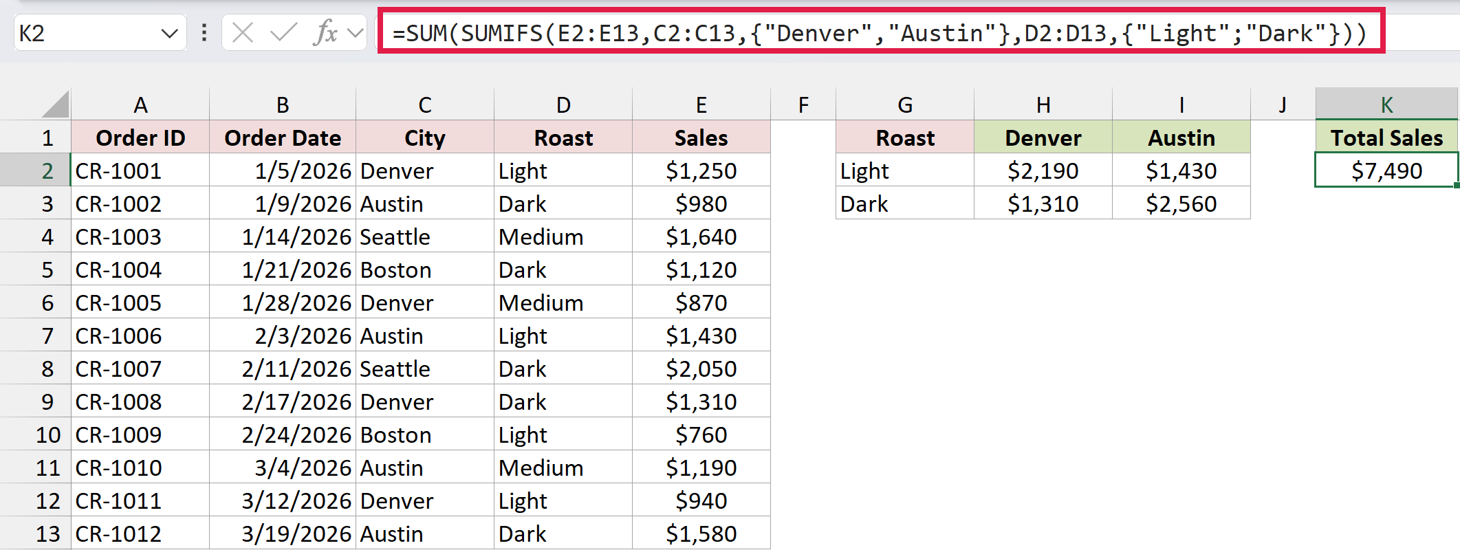
This returns $7,490, the four cells of the grid added together.
The same idea works with cell ranges, and that gives you a quick summary table. I put the roasts down G2:G4, the cities across H1:K1, and entered this formula in H2:
=SUMIFS(E2:E13,D2:D13,G2:G4,C2:C13,H1:K1)
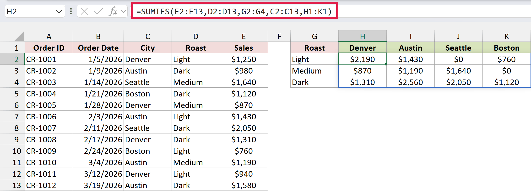
The formula spills a 3-by-4 table with the sales for every roast and city pair. Seattle Light and Boston Medium show $0 because there are no orders for those combinations.
How does this formula work?
When one criteria array is a row and the other is a column, Excel pairs every item in the row with every item in the column. Two cities times two roasts gives four totals, laid out as a grid.
Each cell in that grid is a normal SUMIFS result with two conditions. H2, for example, sums column E where the city is Denver and the roast is Light.
In the cross-tab version, H1:K1 is a row and G2:G4 is a column, so you get the same pairing with real cells. Four cities times three roasts gives twelve totals.
Note: If you use commas in both array constants, like {"Denver","Austin"} and {"Light","Dark"}, Excel doesn’t build a grid. It pairs the items by position (Denver with Light, Austin with Dark), and the SUM version returns $4,750 instead of $7,490.
Method #4: Using a Spill Reference as the Criteria Range
Sometimes the condition isn’t sitting in a column yet. Say you want January sales, but your data only has full dates. SUMIFS won’t take MONTH(B2:B13) as a criteria range, so you need another route.
One way is to spill the calculation into a helper column first. A spill reference points to real cells, so SUMIFS is happy to use it.
Below I have the coffee orders with the order dates in column B. I want the total sales for January.
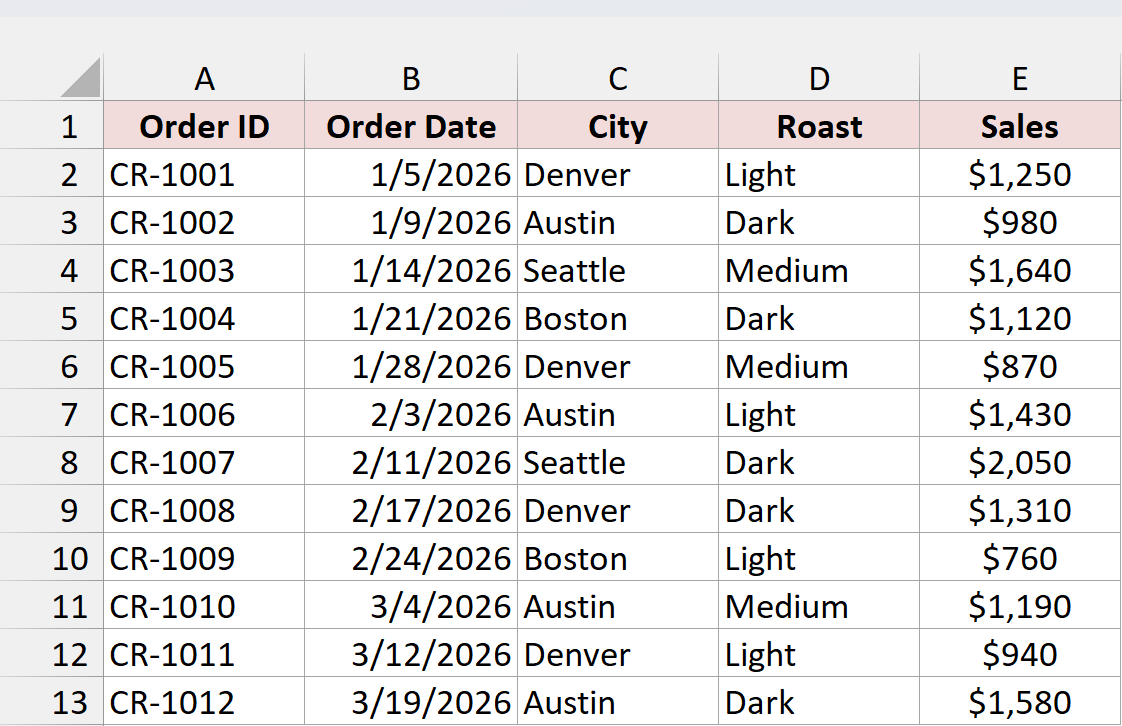
First, I entered this formula in F2 to get the month number for every order:
=MONTH(B2:B13)
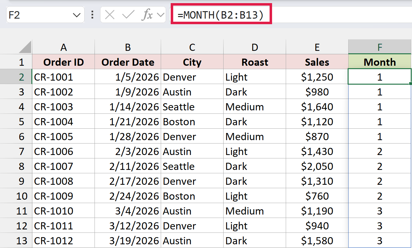
The formula spills down F2:F13 and returns 1 for January, 2 for February, and 3 for March.
Now I can point SUMIFS at that spilled column. Here is the formula I entered in H2:
=SUMIFS(E2:E13,F2#,1)
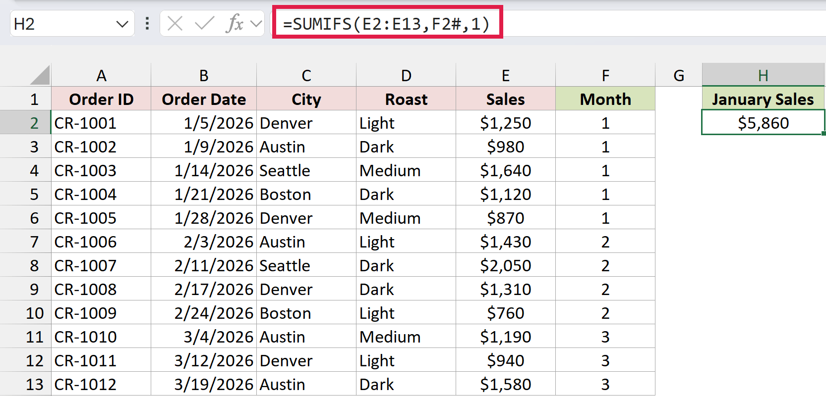
This returns $5,860, the total of the five January orders.
How does this formula work?
The MONTH formula in F2 turns each date into a month number and spills the results into F2:F13.
F2# is a spill reference. The # tells Excel to use the whole spilled range, however many rows it covers. If you add more orders and extend the MONTH formula, F2# grows with it.
Because F2# refers to real cells, SUMIFS treats it like any other criteria range. It sums column E wherever the month number in column F is 1.
Note: Spill references need Excel 2021 or newer (including Microsoft 365). Also, the spilled column has to be the same size as the sum range, or SUMIFS returns a #VALUE! error.
Method #5: Using the SUMPRODUCT Function
If you’d rather not add helper cells, or you need this to work in any version of Excel, SUMPRODUCT is the way to go. It works with arrays everywhere, including calculated ones.
Below I have the same coffee orders. I want the Denver and Austin total from Method #1, and the January total from Method #4.
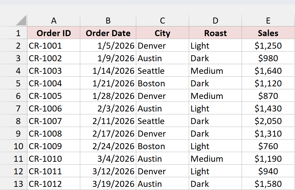
Here is the formula I entered in G2 to get the Denver and Austin total:
=SUMPRODUCT((C2:C13={"Denver","Austin"})*E2:E13)
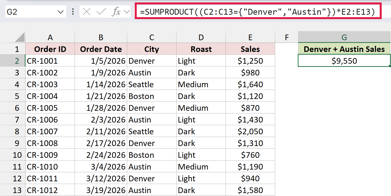
This returns $9,550, the same answer as Method #1.
And here is the formula I entered in G5 to get the January total straight from the dates:
=SUMPRODUCT((MONTH(B2:B13)=1)*E2:E13)
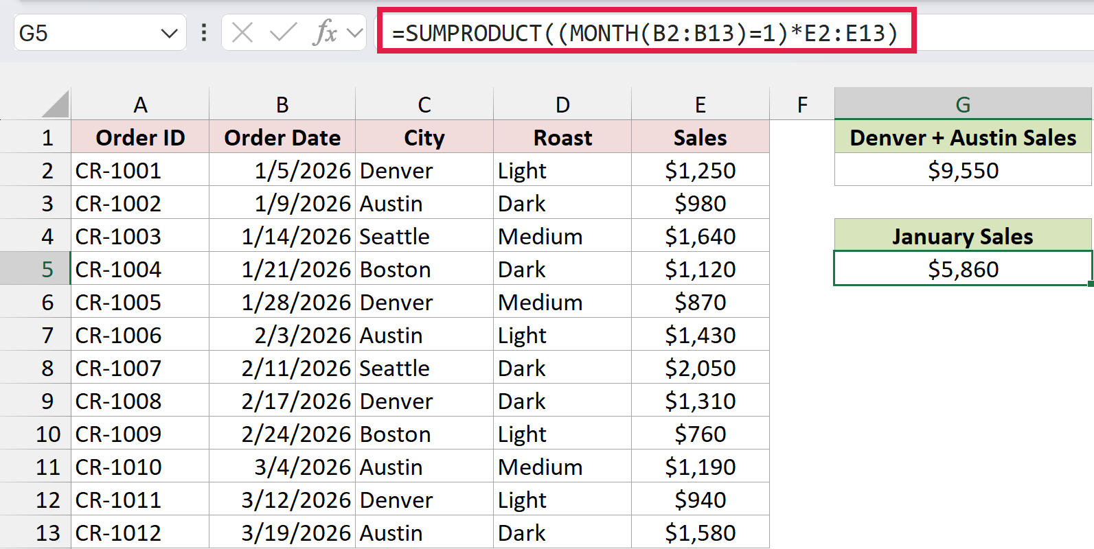
This returns $5,860, the same January total as Method #4, without the helper column.
How does this formula work?
In the first formula, C2:C13={"Denver","Austin"} compares every city with both names. That builds a grid of TRUE and FALSE values, two columns wide and twelve rows tall.
Multiplying by E2:E13 turns TRUE into the sales amount and FALSE into 0. SUMPRODUCT then adds everything up, which gives you the sales for either city.
The second formula works the same way. MONTH(B2:B13)=1 checks each date and returns TRUE for January orders. That’s exactly the calculated array SUMIFS refuses, but SUMPRODUCT handles it without complaint.
Additional Notes About Using SUMIFS With Arrays in Excel
Here are a few things worth keeping in mind when you use arrays with SUMIFS:
- If the same item shows up twice in your list, its total gets added twice.
{"Denver","Denver"}returns $8,740 here, which is double Denver’s real sales. - All the ranges must be the same size. If your sum range is E2:E13 and your criteria range is C2:C9, SUMIFS returns #VALUE!.
- Wildcards work inside array constants.
{"Den*","Aus*"}returns the same $9,550 as the full city names. - The comma and semicolon rules in Method #3 apply to English (US) regional settings. If your Excel uses a comma as the decimal separator, the separators in array constants can be different.
Frequently Asked Questions
Here are some common questions people ask about SUMIFS and arrays.
Can I use an array as the sum range in SUMIFS?
No. The sum range has to be a real range of cells or a spill reference. If you need to sum a calculated array, use SUMPRODUCT, or wrap FILTER in SUM.
Do I need Ctrl + Shift + Enter for these formulas?
Not in Excel 2021 or newer (including Microsoft 365). In Excel 2019 and earlier, the array constant versions work with a normal Enter, but the cell range version in Method #2 needs Ctrl + Shift + Enter.
How do I sum everything except a few values?
Subtract the array total from the grand total. =SUM(E2:E13)-SUM(SUMIFS(E2:E13,C2:C13,{"Denver","Austin"})) returns $5,570, the sales for every city except Denver and Austin.
Can I use FILTER instead of SUMIFS for OR criteria?
Yes, in Excel 2021 or newer (including Microsoft 365). =SUM(FILTER(E2:E13,(C2:C13="Denver")+(C2:C13="Austin"))) returns $9,550. The + between the two tests means a row passes if either one is true.
Does this trick work with COUNTIFS too?
Yes. =SUM(COUNTIFS(C2:C13,{"Denver","Austin"})) returns 8, because there are four Denver orders and four Austin orders.
Conclusion
In this article, I showed you how to use SUMIFS with arrays: array constants and cell ranges as criteria, two arrays that build a grid of totals, a spilled helper column as the criteria range, and SUMPRODUCT for arrays SUMIFS won’t take.
For most OR totals, I’d start with an array constant wrapped in SUM. I hope you found this article helpful.
Other Excel articles you may also like:
- How to Use Criteria in Excel Formulas (With Examples)
- SUMIF vs SUMIFS Function in Excel: What’s the Difference?
- How to Sum Multiple Columns With SUMIFS in Excel
- SUMPRODUCT vs SUMIFS Function in Excel
- How to Use SUMIFS with INDEX MATCH in Excel
- How to Sum Multiple Matching Rows in Excel
- SUMIF Function in Excel
- How to Use SUMIF Across Multiple Sheets in Excel