
When you need to sum multiple matching rows in Excel, VLOOKUP and XLOOKUP return only the first sale for a repeated name.
I’ll use SUMIF for one name, SUMIFS when another column must match too, and SUMPRODUCT for several number columns. GROUPBY or a PivotTable gives you every name’s total.
Sum Matching Rows for One Value
I want to add every sale for one name, even when that name appears in several rows.
Method #1: Using the SUMIF Function
I recommend SUMIF when you want to add up sales for one name. You can use it in every Excel version.
Below I have a dataset of orders with sales reps, regions, and sales amounts. I want Maria’s total, with her name in F2 and the answer in G2.
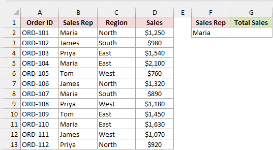
If you enter =VLOOKUP("Maria",B2:D13,3,FALSE), you’ll get $1,250, Maria’s first order. Her four orders actually total $5,870.
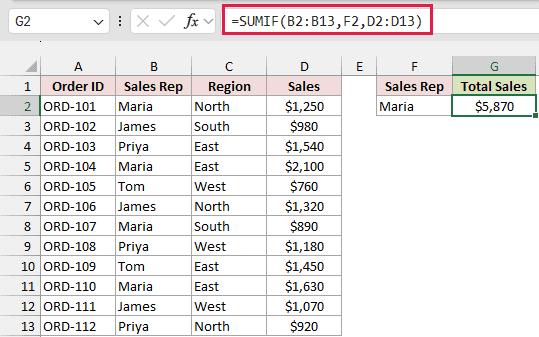
Here is the formula to enter in G2:
=SUMIF(B2:B13,F2,D2:D13)
How does this formula work?
I’m using the sales rep’s name to decide which sales to add. Excel adds each sale whose name matches Maria.
B2:B13contains the names you want to check.F2contains the name to match, Maria.D2:D13contains the sales amounts you want to add.
You’ll get the sales from Maria’s four rows: $1,250 + $2,100 + $890 + $1,630 = $5,870.
Because I used F2 instead of typing Maria into the formula, you can change the name there. Type James, and you’ll get $3,370.
Method #2: Using the SUMIFS Function
Sometimes you need more than the name to match. I want Maria’s sales in the East region only, so I’ll use SUMIFS.
Below I have orders with sales reps, regions, and sales amounts, plus Maria in F2 and East in G2.
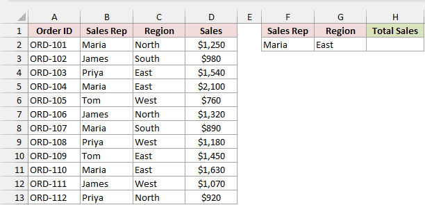
H2 is where the total goes. Enter this formula:
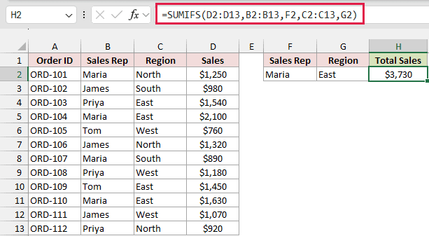
=SUMIFS(D2:D13,B2:B13,F2,C2:C13,G2)
How does this formula work?
With this formula, I add a sale only when both the sales rep and the region match.
D2:D13is the range to add. With SUMIFS, you put this first. With SUMIF, you put it last.B2:B13,F2checks whether the sales rep is Maria.C2:C13,G2checks whether the region is East.
You only add a row when both checks match. That’s called AND logic, and you can add more range-and-value pairs for additional checks.
You’ll get $3,730 from ORD-104 and ORD-110: $2,100 + $1,630. Maria’s orders in other regions stay out of this total.
Method #3: Using the SUMPRODUCT Function
So far, you’ve added one sales column. When each matching row has several number columns, you can add them all with SUMPRODUCT.
Below I have a dataset of monthly sales by rep and region. I want Maria’s January-to-March total, with her name in G2 and the answer in H2.
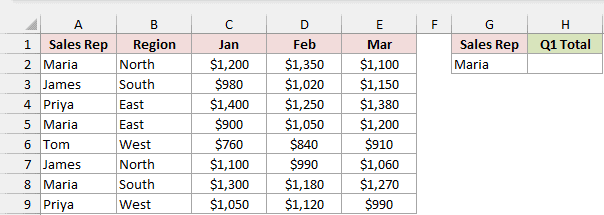
Enter this formula in H2:
=SUMPRODUCT((A2:A9=G2)*C2:E9)
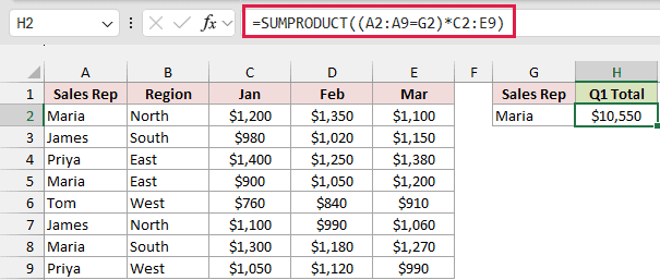
You can press Enter normally. You don’t need Ctrl + Shift + Enter in any Excel version.
How does this formula work?
I keep all three monthly amounts for Maria’s rows and replace the other reps’ amounts with zero.
A2:A9=G2checks the name in each of the eight rows against Maria. You get TRUE for her rows and FALSE for the others.- Multiplying that check by
C2:E9turns TRUE into 1 and FALSE into 0. Maria’s monthly amounts remain, and everyone else’s become 0. - SUMPRODUCT adds all the remaining amounts across the three columns.
You’ll get $10,550 from Maria’s three row totals: $3,650 + $3,150 + $3,750.
To include only Maria’s East row, add another check: =SUMPRODUCT((A2:A9=G2)*(B2:B9="East")*C2:E9). You’ll get $3,150.
Note: You can’t get this total by giving SUMIF several sales columns. =SUMIF(A2:A9,"Maria",C2:E9) returns $3,400, only Maria’s January sales. SUMIF resizes the sum range to match the one-column names range, so you get an incomplete total without an error.
A word such as “N/A” in the number block gives #VALUE! with this SUMPRODUCT formula. SUMIF and SUMIFS skip text instead.
Get a Total for Every Matching Value
I want a separate total for each sales rep, with all their matching rows combined.
Method #4: Using the GROUPBY Function
When you want everyone’s totals, you don’t have to write a separate SUMIF for each name. In Excel for Microsoft 365, you can use GROUPBY.
Below I have a dataset of orders with sales reps, regions, and sales amounts. I want one summary row for each rep’s total sales.
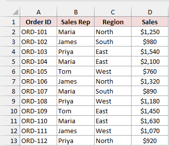
First, type Sales Rep in F1 and Total Sales in G1. Enter this formula in F2:
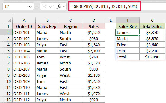
=GROUPBY(B2:B13,D2:D13,SUM)
How does this formula work?
To summarize every rep, I group their orders and add the sales amounts. You get the whole summary from one formula.
B2:B13contains the names to group together. Each rep appears once in your summary.D2:D13contains the sales amounts to add.SUM, typed without parentheses, tells Excel to add the amounts within each group.
You’ll see the results spread into F2:G6 automatically. This is called spilling.
You get the names sorted A to Z, followed by a Total row:
- James: $3,370.
- Maria: $5,870.
- Priya: $3,640.
- Tom: $2,210.
- Total: $15,090.
Your summary updates when you change a value in B2:B13 or D2:D13. Rows you add below row 13 aren’t included.
If you want only the reps, without the Total row, use =GROUPBY(B2:B13,D2:D13,SUM,,0).
If you don’t have GROUPBY, you can get the same totals with a PivotTable below.
Method #5: Using a PivotTable
If you’d rather click than type a formula, you can group the matching orders into a summary with a PivotTable. This works in every Excel version.
Below I have a dataset of orders with each sale’s rep and region. I want a separate sales total for every rep.
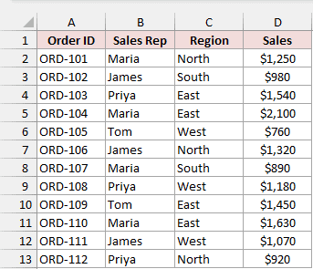
Here are the steps to combine the matching rows and sum each rep’s sales:
- Select any cell inside the dataset.
- Click the Insert tab, then click PivotTable. In the PivotTable from table or range dialog, you’ll see the data range filled in and New Worksheet selected. In older versions, the dialog is called Create PivotTable.
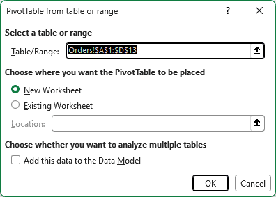
- Keep New Worksheet selected and click OK. You’ll get a new sheet with an empty PivotTable and the PivotTable Fields pane on the right.
- In the PivotTable Fields pane, check Sales Rep and then Sales. You’ll see Sales Rep in Rows and Sum of Sales in Values.
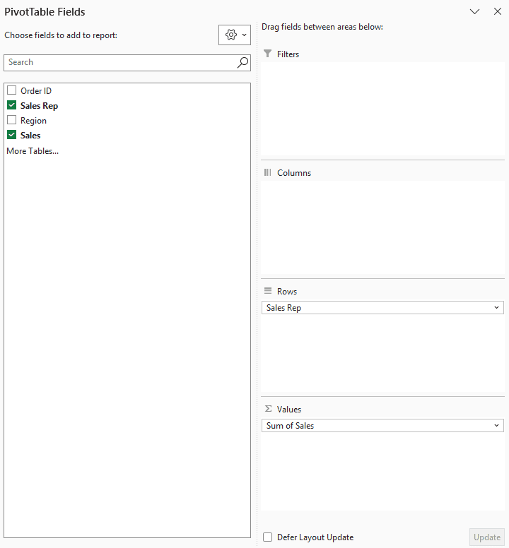
You’ll now have a sales total for each rep under Row Labels and Sum of Sales, followed by a Grand Total.
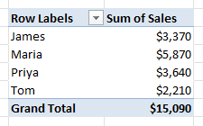
Your totals are James $3,370, Maria $5,870, Priya $3,640, and Tom $2,210. The Grand Total is $15,090.
You’ll see dollar signs here because I set the number format. A new PivotTable shows plain numbers, such as 3370, by default.
To match this format, right-click any total, click Number Format, choose Currency, set Decimal places to 0, and click OK.
After you change the source data, right-click the PivotTable and click Refresh. You can also use Refresh All on the Data tab.
Note: Before you insert the PivotTable, convert your source data to an Excel Table with Ctrl + T. Then new rows you add to the Table are included when you refresh the PivotTable.
Additional Notes About Summing Matching Rows in Excel
- Wrapping a lookup in SUM won’t add the other matching rows. SUM receives just one result from VLOOKUP, XLOOKUP, or INDEX MATCH.
- Numbers stored as text can leave you with a low total. If Maria’s $1,250 sale in D2 is text, SUMIF returns $4,620. Check for left-aligned numbers.
- If F2 holds
"Maria "with a trailing space, SUMIF returns 0. Use TRIM to remove extra spaces from names or your lookup cell.
Frequently Asked Questions
Here are a few other ways you might want to match names or narrow down the sales you add.
How do I sum rows that match one name or another in Excel?
To add Maria’s sales and Tom’s sales together, use =SUM(SUMIF(B2:B13,{"Maria","Tom"},D2:D13)). You’ll get $8,080.
SUMIF returns a separate total for each name. SUM adds those totals together, so a row can match either name.
Is SUMIF case-sensitive?
No. You can use "maria" instead of "Maria" and still get $5,870. Capital letters don’t change which names match.
How do I sum matching rows with FILTER in Excel 365?
You can keep only Maria’s sales and then add them with =SUM(FILTER(D2:D13,B2:B13="Maria")). You’ll get $5,870, the same total as SUMIF.
FILTER returns the sales from Maria’s rows. SUM adds those returned amounts.
How do I sum matching rows only when sales are over a limit?
To add Maria’s orders over $1,000, use =SUMIFS(D2:D13,B2:B13,"Maria",D2:D13,">1000"). You’ll get $4,980.
You’re adding $1,250 + $2,100 + $1,630. Maria’s $890 order is below the limit, so you leave it out.
Conclusion
For one name, I’d start with SUMIF and use SUMIFS when another column also needs to match.
I’d use SUMPRODUCT to add several number columns for each matching row. For every name’s total, choose GROUPBY or a PivotTable.
Other Excel articles you may also like:
- How to Sum Multiple Columns With SUMIFS in Excel
- How to Use SUMIFS with INDEX MATCH in Excel
- How to Use VLOOKUP with Multiple Criteria in Excel
- How to Use SUMIF Across Multiple Sheets in Excel
- SUMPRODUCT vs SUMIFS Function in Excel
- SUMIF vs SUMIFS Function in Excel: What’s the Difference?
- How to Use Criteria in Excel Formulas (With Examples)
- How to Sum Every N Rows in Excel
