
Criteria in Excel formulas let you count or add only the entries you need, such as paid bookings or prices above a limit.
You write the condition differently depending on what you’re checking: text needs quotes, while a comparison with a cell needs an ampersand.
You can also combine conditions to narrow your results or include several categories.
I’ll show you how to write criteria that pick the entries you want in an Excel formula.
How Criteria Work in Excel Formulas
When you want a formula to count, sum, or average only certain cells, you give it a condition. That condition is its criteria argument.
You can use a criteria argument with these functions:
- COUNTIF: count cells meeting one condition.
- COUNTIFS: count cells meeting multiple conditions.
- SUMIF: add values meeting one condition.
- SUMIFS: add values meeting multiple conditions.
- AVERAGEIF: average values meeting one condition.
- AVERAGEIFS: average values meeting multiple conditions.
- MAXIFS: find the largest value meeting your conditions.
- MINIFS: find the smallest value meeting your conditions.
You’ll need Excel 2019 or later (or Microsoft 365) for MAXIFS and MINIFS.
Put text inside double quotes, such as "Miami". You can enter a number directly, such as 500, without quotes.
For a comparison, put the operator and value together inside quotes. For example, ">1000" means greater than 1000.
Here are the comparison operators you can use:
| Operator | Meaning | Example criteria |
|---|---|---|
= | Equal to | "=Paid" |
> | Greater than | ">1000" |
< | Less than | "<500" |
>= | Greater than or equal to | ">=500" |
<= | Less than or equal to | "<=500" |
<> | Not equal to | "<>Refunded" |
If your comparison value is in a cell, join the quoted operator to the reference with &, like this: ">="&J1.
Example #1: Using Text Criteria
You can count entries that match a city, payment status, or another piece of text. I’ll start by counting bookings to Miami.
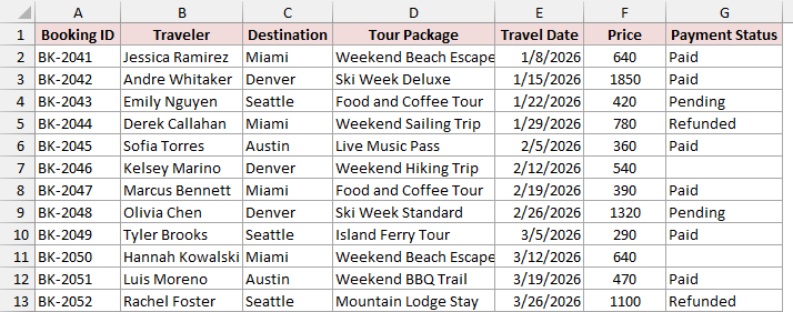
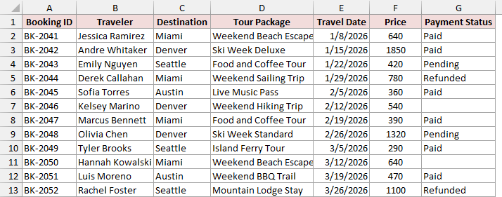
Below I have a dataset of 12 travel bookings in A1:G13, with headers in row 1 and bookings in rows 2 through 13.
You can see each booking’s ID, traveler, destination, tour package, travel date, price, and payment status.
To count Miami bookings, I entered Miami Bookings in I1 and this formula in J1:
=COUNTIF(C2:C13,"Miami")
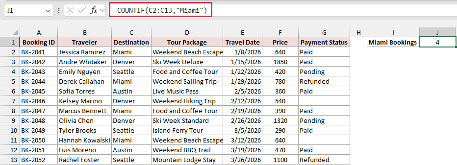
You get 4 in J1 because four bookings have Miami as their destination.
How does this formula work?
I use C2:C13 to tell COUNTIF where to look. The criteria "Miami" tells it which text to count.
You need double quotes around the text. You don’t need to match its capitalization: "miami" also returns 4.
Example #2: Using Comparison Operators
Now let’s count or add entries based on a comparison, such as a price above a limit or a status you want to exclude.
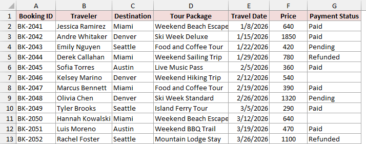
Below I have a dataset of 12 travel bookings in A1:G13. You can see their prices in column F and payment statuses in column G.
To add prices greater than 1000, I entered Total of Prices Over 1000 in I1 and this formula in J1:
=SUMIF(F2:F13,">1000")
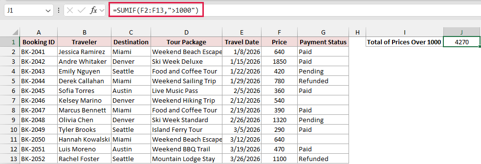
You get 4270 in J1, the total of 1850, 1320, and 1100.
How does this formula work?
I use ">1000" to include only prices above 1000. A price equal to 1000 wouldn’t qualify.
Because I’m checking and adding the same range, F2:F13, I can leave out SUMIF’s third argument.
You can also exclude a particular status. I entered Bookings Not Refunded in I2 and this formula in J2:
=COUNTIF(G2:G13,"<>Refunded")
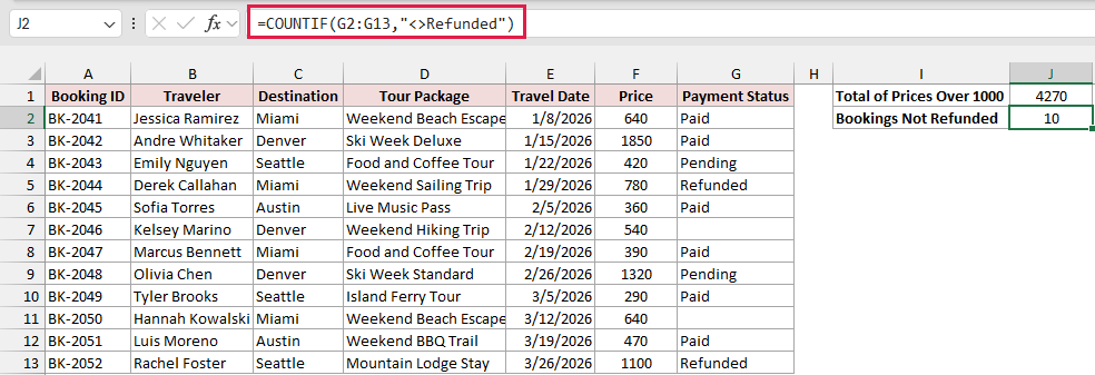
You get 10 in J2.
How does this formula work?
I put <> before Refunded to mean “not equal to Refunded.” You count every booking whose status isn’t Refunded, including the two blank statuses.
Note: To exclude blank statuses too, use =COUNTIFS(G2:G13,"<>Refunded",G2:G13,"<>"). You get 8 instead of 10.
Example #3: Using a Cell Reference as Criteria
Instead of editing your formula whenever a limit changes, you can keep that limit in a cell. I’ll use a minimum booking price.
Below I have a dataset of 12 travel bookings in A1:G13, with prices in column F.
You can also see Minimum Price in I1 and the value 500 in J1.
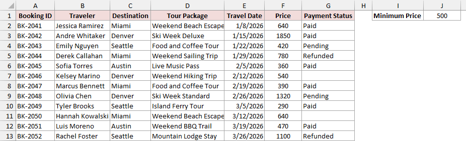
To count prices at or above that minimum, I entered Bookings at or Above Minimum in I2 and this formula in J2:
=COUNTIF(F2:F13,">="&J1)
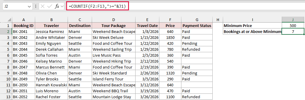
You get 7 in J2.
How does this formula work?
I use & to join the operator ">=" to the value in J1. With 500 in that cell, the resulting condition is ">=500".
Keep J1 outside the quotes. If you write ">=J1", Excel treats J1 as literal text, and you get 0 on this dataset.
Change the minimum in J1, and your count updates. I use this approach when a report needs a limit you can adjust.
When you use an empty cell directly as criteria, Excel treats it as 0, so it doesn’t match blank cells.
For example, =COUNTIF(G2:G13,M1) returns 0 when M1 is empty. It doesn’t count the two blank payment statuses.
Example #4: Using Wildcards for Partial Matches
You don’t always need to match an entire name. Here, I’ll add prices for every tour package whose name starts with Weekend.
Below I have a dataset of 12 travel bookings in A1:G13. You can see the tour package names in column D and prices in column F.
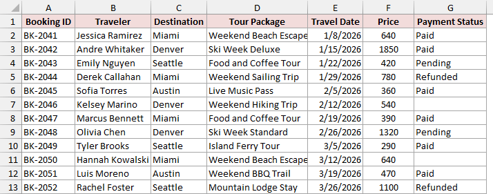
To total those packages, I entered Weekend Package Sales in I1 and this formula in J1:
=SUMIF(D2:D13,"Weekend*",F2:F13)
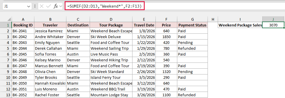
You get 3070 in J1 from five Weekend packages: 640 + 780 + 540 + 640 + 470.
How does this formula work?
I use "Weekend*" to match Weekend followed by any text. SUMIF checks the package names in D2:D13 and adds matching prices from F2:F13.
The asterisk is a wildcard. You have three wildcard patterns to work with:
*matches any number of characters. Use"*Tour*"to match text containing Tour anywhere.?matches exactly one character."BK-204?"matches BK-2041 through BK-2049, so=COUNTIF(A2:A13,"BK-204?")returns 9.~before*or?matches the literal character. For example,"~*"matches an actual asterisk.
You can use wildcards to match text, but they don’t match numeric values.
Example #5: Using Dates as Criteria
Next, I’ll use a date as the cutoff. You can count trips from a particular day or add prices within a whole month.
Below I have a dataset of 12 travel bookings in A1:G13. The travel dates in column E run from January 8 through March 26, 2026.
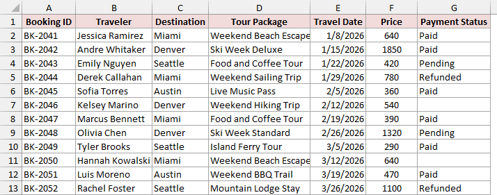
To count trips on or after March 1, 2026, I entered Trips On or After Mar 1 in I1 and this formula in J1:
=COUNTIF(E2:E13,">="&DATE(2026,3,1))
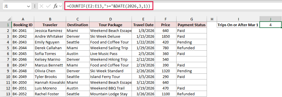
You get 4 in J1.
How does this formula work?
I use DATE(2026,3,1) to specify March 1, 2026, then join it to ">=". Your condition includes that day and every later date.
If you type ">=3/1/2026" instead, Excel interprets the date using your computer’s regional settings. DATE specifies the same day regardless of those settings.
You can also join the operator to a cell containing a date, or to TODAY() when you want the cutoff to be today’s date.
To add prices for February trips, I entered February Sales in I2 and this formula in J2:
=SUMIFS(F2:F13,E2:E13,">="&DATE(2026,2,1),E2:E13,"<"&DATE(2026,3,1))
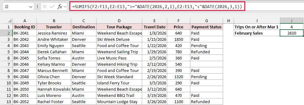
You get 2610 in J2.
How does this formula work?
I check E2:E13 twice: once for dates on or after February 1, and once for dates before March 1. SUMIFS adds the corresponding prices.
Using the first day of the next month works for any month length. You don’t need to work out its final day.
It also counts dates that include a time on the month’s last day. A "<=" cutoff at February 28 would exclude times after midnight that day.
Example #6: Checking for Blank and Non-Blank Cells
You can also check for missing entries. I’ll count bookings awaiting a payment status, then count those with a status entered.
Below I have a dataset of 12 travel bookings in A1:G13. The Payment Status cells for BK-2046 and BK-2050 are blank.
To count the missing statuses, I entered Missing Payment Status in I1 and this formula in J1:
=COUNTIF(G2:G13,"")
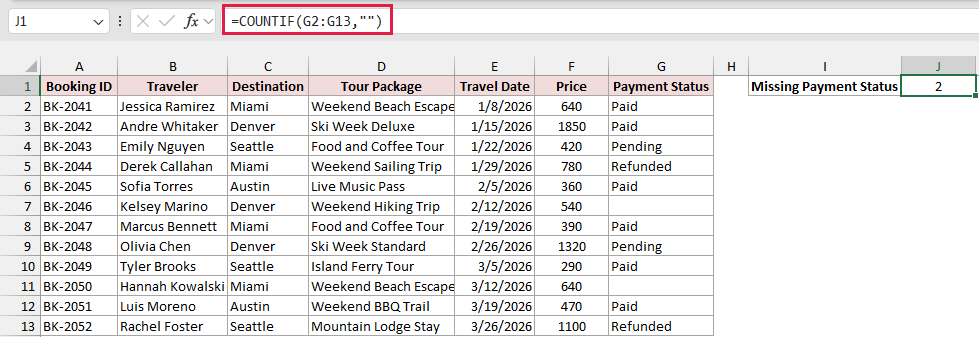
You get 2 in J1.
How does this formula work?
I use two double quotes with nothing between them, "", to count blank payment statuses in G2:G13.
For bookings with a status entered, I entered Payment Status Entered in I2 and this formula in J2:
=COUNTIF(G2:G13,"<>")
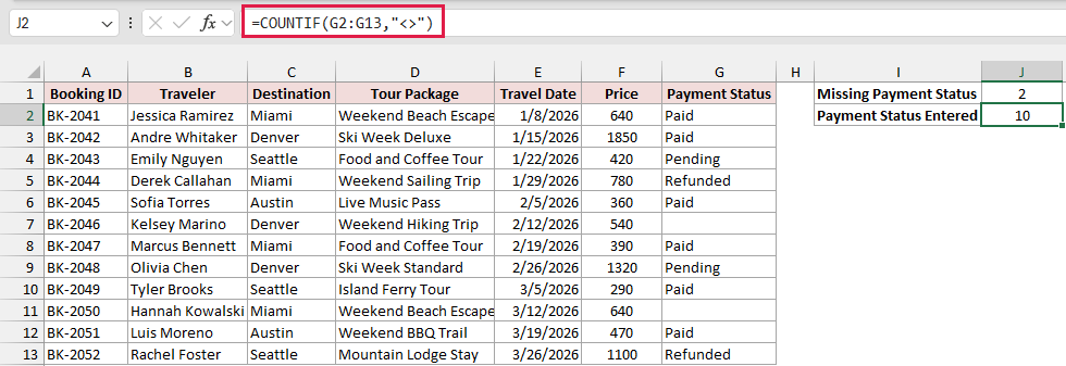
You get 10 in J2.
How does this formula work?
I use "<>" to count cells with an entry. Here, you have ten cells containing Paid, Pending, or Refunded.
You count a formula returning empty text ("") with both "" and "<>". To match only truly empty cells, use "=".
Example #7: Using Multiple Criteria (AND Logic)
Let’s narrow the total using two conditions. I’ll add prices only when the destination is Miami and the payment status is Paid.
Below I have a dataset of 12 travel bookings in A1:G13, with destinations in column C, prices in column F, and payment statuses in column G.
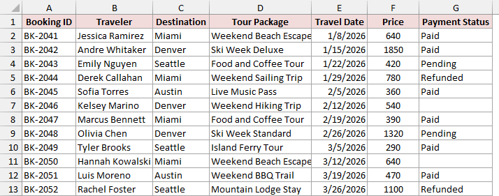
To total paid Miami bookings, I entered Paid Miami Sales in I1 and this formula in J1:
=SUMIFS(F2:F13,C2:C13,"Miami",G2:G13,"Paid")
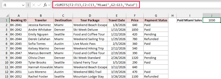
You get 1030 in J1, the total of 640 and 390.
How does this formula work?
I put the sum range, F2:F13, first. After that, I supply a range and its criteria for each condition.
You include a price only when both conditions are true. That’s AND logic: the destination must be Miami, and the status must be Paid.
Keep all your ranges the same size. Ranges of different sizes give you a #VALUE! error.
You can apply the same range-and-criteria pairing with COUNTIFS, AVERAGEIFS, MAXIFS, and MINIFS. Every condition must be met there too.
Example #8: Using Multiple Criteria (OR Logic)
Sometimes you want either condition to qualify. I’ll add prices for bookings that are Pending or Refunded, using one total for both statuses.
Below I have a dataset of 12 travel bookings in A1:G13. You can see payment statuses in column G and the corresponding prices in column F.
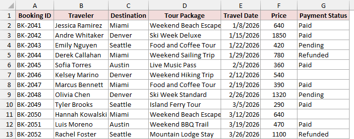
To combine those totals, I entered Pending or Refunded Total in I1 and this formula in J1:
=SUM(SUMIF(G2:G13,{"Pending","Refunded"},F2:F13))
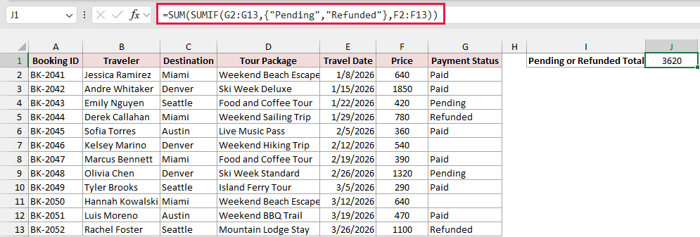
You get 3620 in J1: 1740 for Pending bookings plus 1880 for Refunded bookings.
How does this formula work?
I put both statuses inside curly braces. This list, called an array constant, makes SUMIF calculate a separate total for each status.
SUM then adds those two totals. You include a booking when either status matches, which is OR logic.
In Microsoft 365, leaving out SUM would spill the two separate totals into two cells instead of combining them.
You can also use this formula in older Excel versions. You don’t need Ctrl+Shift+Enter because the criteria come from an array constant.
If you prefer, add two SUMIF formulas: =SUMIF(G2:G13,"Pending",F2:F13)+SUMIF(G2:G13,"Refunded",F2:F13).
Example #9: Using Logical Tests in FILTER and SUMPRODUCT
With FILTER and SUMPRODUCT, you use logical tests instead of criteria strings. You can return matching booking IDs or test a calculation on each date.
Below I have a dataset of 12 travel bookings in A1:G13, with booking IDs in column A, destinations in C, dates in E, and prices in F.
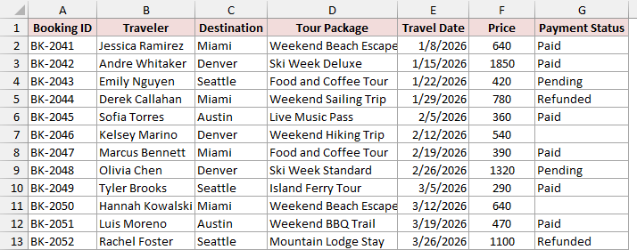
To list Denver bookings priced above 1000, I entered Denver Bookings Over 1000 in I1 and this formula in I2:
=FILTER(A2:A13,(C2:C13="Denver")*(F2:F13>1000))
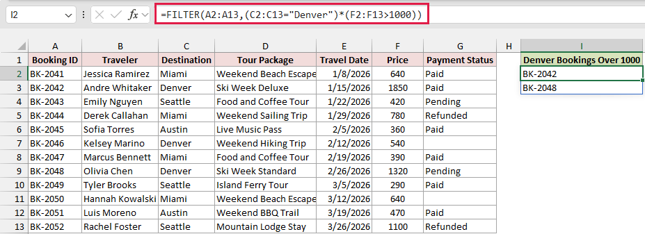
You get BK-2042 in I2 and BK-2048 in I3. The formula spills down the column automatically.
How does this formula work?
I compare each destination with Denver and each price with 1000. Each comparison returns TRUE or FALSE for every booking.
Multiplying the tests with * keeps bookings where both are true. You can use + between tests for OR logic instead.
FILTER returns the matching booking IDs from A2:A13. You’ll need Microsoft 365 or Excel 2021 or later to use it.
With FILTER and SUMPRODUCT, you write logical tests such as C2:C13="Denver", rather than criteria strings such as ">1000".
COUNTIF needs a real cell range, so Excel rejects =COUNTIF(UPPER(C2:C13),"MIAMI"). You can’t use UPPER(C2:C13) as its criteria range.
With logical tests, you can calculate values first, then check them against your condition.
On a separate sheet with the same bookings, I entered March Sales in I1 and this formula in J1 to total March trips:
=SUMPRODUCT((MONTH(E2:E13)=3)*F2:F13)
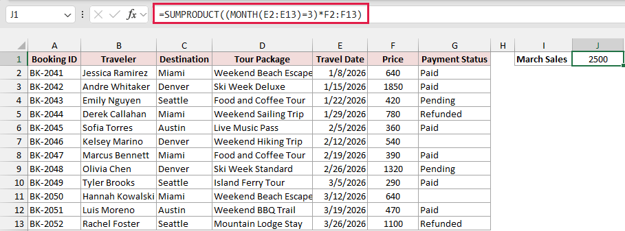
You get 2500 in J1.
How does this formula work?
I use MONTH to calculate the month number for every travel date. The test =3 identifies March, and multiplication keeps only those booking prices.
SUMPRODUCT adds the resulting values. You can use it in every Excel version.
You can’t put MONTH(E2:E13) directly into a SUMIFS criteria range. SUMPRODUCT lets you perform that calculation before testing each value.
Additional Notes About Using Criteria in Excel Formulas
Before you reuse these patterns with your own data, I recommend checking these details:
- If capitalization must affect your result, use EXACT with SUMPRODUCT. Ordinary criteria matching won’t distinguish uppercase from lowercase.
- Keep criteria text within 255 characters. Longer strings can produce incorrect COUNTIF results or a
#VALUE!error. - If your text contains double quotes, double those quotes inside the criteria string. You can instead put the text in a cell and reference it.
Frequently Asked Questions
Here are a few questions you might have when adapting these formulas to your own worksheet.
Can I use OR criteria in COUNTIFS?
Yes. Use =SUM(COUNTIFS(G2:G13,{"Pending","Refunded"})) to count bookings with either status. You get 4 on this data.
Alternatively, add the two counts with =COUNTIF(G2:G13,"Pending")+COUNTIF(G2:G13,"Refunded").
Why does my COUNTIF return 0 when the text looks correct?
Check for extra spaces in your data. A cell containing Miami won’t match "Miami", even though the trailing space can be hard to spot.
Can Excel criteria refer to another sheet?
Yes. Keep the operator in quotes and join the other sheet’s reference, such as ">="&Sheet2!B1. Your threshold can live on a separate settings sheet.
Conclusion
I recommend starting with criteria strings in COUNTIFS or SUMIFS, and keeping any condition you’ll change in a cell you can reference.
When your condition needs a calculation, reach for FILTER to return matching entries or SUMPRODUCT to calculate a total.
Other Excel articles you may also like:
- SUMPRODUCT vs SUMIFS Function in Excel
- SUMIF vs SUMIFS Function in Excel: What’s the Difference?
- How to Sum Multiple Columns With SUMIFS in Excel
- How to COUNTIF Partial Match in Excel?
- Count Cells Less than a Value in Excel (COUNTIF Less)
- How to Use Greater Than or Equal to Operator in Excel Formula?
- Using Less Than or Equal to Operator in Excel Formula
- How to Use VLOOKUP with Multiple Criteria in Excel
