
Monthly sales sheets in Excel often share the same layout, but you still need one total per drink across all those months.
Using SUMIF across multiple sheets seems straightforward until a reference like SUMIF(Jan:Mar!...) returns #VALUE!.
SUMIF can’t read that kind of reference, so you need to add separate calculations or combine the data first.
I’ll show you six ways to do this, from a simple SUMIF formula to Power Query.
Method #1: Using SUMIF for Each Sheet
For a few sheets, I find it easiest to calculate each month’s total with SUMIF, then add those totals together.
Below I have the Jan sheet with ten coffee catering orders. Feb and Mar have the same layout.
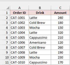
Column B contains the drink names, and column C contains the amounts. I want the combined sales for each drink across all three months.
On a summary sheet, type Drink in A1 and list Latte, Cold Brew, Mocha, Cappuccino, and Americano in A2:A6.
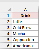
Type Total Sales in B1. In Excel with dynamic arrays, enter this formula in B2 and leave B3:B6 empty for the results:
=SUMIF(Jan!B2:B11,A2:A6,Jan!C2:C11)+SUMIF(Feb!B2:B11,A2:A6,Feb!C2:C11)+SUMIF(Mar!B2:B11,A2:A6,Mar!C2:C11)
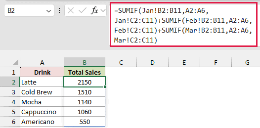
The formula spills down B2:B6 automatically. It returns 2150 for Latte, 1510 for Cold Brew, 1140 for Mocha, 1060 for Cappuccino, and 550 for Americano.
How does this formula work?
The first SUMIF checks Jan!B2:B11 for each drink in A2:A6 and adds the matching amounts from Jan!C2:C11.
For Latte, that first calculation returns 750. The other two SUMIF calculations do the same for Feb and Mar.
The plus signs add the three monthly totals for each drink. Passing A2:A6 as the criteria lets one formula return all five results.
You need another SUMIF for every extra sheet, so this formula gets long when you have many months.
Note: In Excel 2019 and older, enter =SUMIF(Jan!$B$2:$B$11,A2,Jan!$C$2:$C$11)+SUMIF(Feb!$B$2:$B$11,A2,Feb!$C$2:$C$11)+SUMIF(Mar!$B$2:$B$11,A2,Mar!$C$2:$C$11) in B2 and copy it down to B6. This version calculates one drink at a time, with the source ranges fixed.
Method #2: Using VSTACK and FILTER
For Microsoft 365 or Excel 2024, this is the method I recommend. The formula stays short however many monthly sheets you include.
Below I have the Jan sheet with drink names and order amounts. Feb and Mar use the same columns and rows.
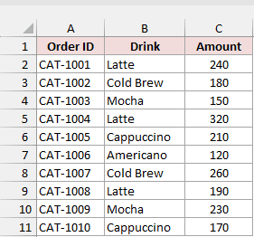
I want the total sales for each drink across Jan, Feb, and Mar. VSTACK combines their data so FILTER can select the matching orders.
On a summary sheet, type Drink in A1 and list Latte, Cold Brew, Mocha, Cappuccino, and Americano in A2:A6.
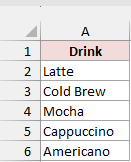
Type Total Sales in B1. Enter the following formula in B2, then copy it down to B6:
=SUM(FILTER(VSTACK(Jan:Mar!$C$2:$C$11),VSTACK(Jan:Mar!$B$2:$B$11)=A2,0))
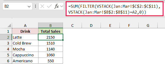
B2 returns 2150 for Latte. The remaining rows return 1510, 1140, 1060, and 550 for the other drinks.
How does this formula work?
VSTACK(Jan:Mar!$C$2:$C$11) stacks the amounts from the three sheets into one 30-row list. Unlike SUMIF, VSTACK accepts a reference spanning several sheets.
Excel rejects VSTACK inside SUMIF because SUMIF needs a real range, so FILTER and SUM handle the matching and adding instead.
The second VSTACK builds a matching list of drink names. Comparing that list with A2 picks out the Latte orders.
FILTER keeps the amounts for those matching orders. Its third argument, 0, returns zero instead of #CALC! when the drink has no orders.
SUM adds the filtered amounts into one total. Because SUM returns one value, I copy this formula down to calculate the other drinks.
Keep the $ signs exactly as shown. They hold the source ranges in place when you copy down, while A2 changes to the next drink.
Note: Keep your summary sheet outside the Jan-to-Mar tab range. The formula includes every sheet between those two tabs, so inserting another monthly sheet between them includes it automatically.
Method #3: Using SUMPRODUCT, SUMIF, and INDIRECT
When you want to choose sheets from a list, this combination works in every Excel version.
Below I have the Jan sheet with ten orders and their amounts. Feb and Mar have the same layout.
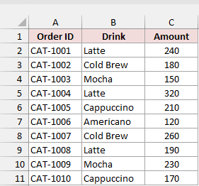
I want a total for each drink across the three months, using sheet names typed on the summary sheet.
Type Drink in A1 and list Latte, Cold Brew, Mocha, Cappuccino, and Americano in A2:A6. Type Total Sales in B1 and leave B2:B6 empty.
In D1, type Sheet Names. Enter Jan, Feb, and Mar in D2:D4, one name per cell.
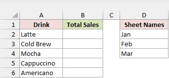
Enter this formula in B2, then copy it down to B6. SUMPRODUCT returns one combined total for the drink in each row:
=SUMPRODUCT(SUMIF(INDIRECT("'"&$D$2:$D$4&"'!B2:B11"),A2,INDIRECT("'"&$D$2:$D$4&"'!C2:C11")))
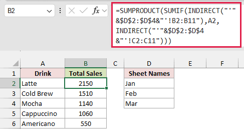
The totals are 2150 for Latte, 1510 for Cold Brew, 1140 for Mocha, 1060 for Cappuccino, and 550 for Americano.
How does this formula work?
The first INDIRECT builds references from the names in D2:D4. For Jan, it turns the text 'Jan'!B2:B11 into a reference to the drink cells.
The second INDIRECT does the same for the amount cells in C2:C11. The single quotes around each sheet name keep it working for names with spaces.
SUMIF calculates a separate total for each listed sheet, using A2 as the drink to match. SUMPRODUCT adds those three numbers together.
To include another sheet, add its name to the list and extend $D$2:$D$4 in both places. A blank cell inside that range breaks the formula.
The references inside INDIRECT are text, so they won’t adjust if you insert rows on the monthly sheets. Update those text ranges when needed.
Note: INDIRECT is volatile, which means it recalculates on every change. This can slow down a large workbook, especially when you use many formulas like this.
Method #4: Using GROUPBY With VSTACK
If you have Microsoft 365, GROUPBY can build the whole drink summary for you, including the names and a grand total.
Below I have the Jan sheet with drink names in column B and amounts in column C. Feb and Mar have the same layout.
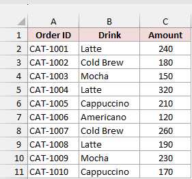
I want one summary of sales across all three months. Here, you don’t need to type a list of drinks first.
On an empty summary sheet, type Drink in A1 and Total Sales in B1. Leave A2:B7 clear, then enter this formula in A2:
=GROUPBY(VSTACK(Jan:Mar!B2:B11),VSTACK(Jan:Mar!C2:C11),SUM)
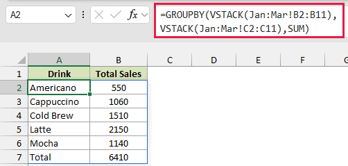
The formula spills into A2:B7. GROUPBY lists the drinks alphabetically and adds a Total row automatically:
- Americano: 550
- Cappuccino: 1060
- Cold Brew: 1510
- Latte: 2150
- Mocha: 1140
- Total: 6410
How does this formula work?
The first VSTACK combines the drink names from Jan through Mar. The second combines the matching amounts.
GROUPBY groups the amounts by drink name, then uses SUM to calculate each group’s total. It returns both columns, so there’s no formula to copy down.
The final Total row adds all the drink totals together, returning 6410 for the three months.
Note: GROUPBY needs Microsoft 365. It isn’t available in Excel 2024, even though Excel 2024 supports VSTACK.
Method #5: Using the Consolidate Feature
If you’d prefer to use Excel’s menus, Consolidate can add the amounts for matching drink labels across your monthly sheets.
Below I have the Jan sheet with Order ID, Drink, and Amount columns. Feb and Mar have the same layout.
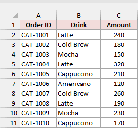
I want a combined sales total for each drink. For this method, select only the Drink and Amount columns from each month.
Consolidate uses the left column of each selected range as its labels. Including Order ID would make it group by order instead of drink.
Here are the steps to combine the monthly sales:
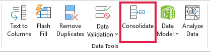
- Select A1 on a blank summary sheet. On the Data tab, in the Data Tools group, click Consolidate. The output will start at A1.
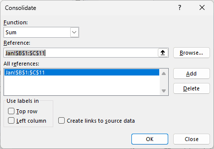
- Set Function to Sum. Click in the Reference box, go to Jan, and select B1:C11, including the headers. Click Add. The All references list now contains
Jan!$B$1:$C$11.
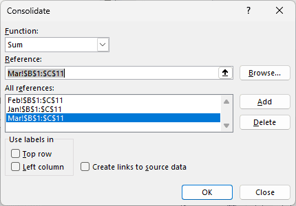
- Repeat the reference selection for Feb and Mar, clicking Add after each one. The list should contain
Jan!$B$1:$C$11,Feb!$B$1:$C$11, andMar!$B$1:$C$11.
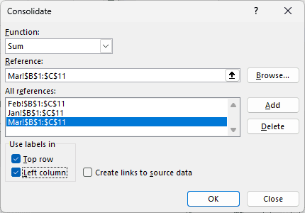
- Under Use labels in, check Top row and Left column. For this example, leave Create links to source data unchecked.
- Click OK. Excel leaves A1 empty, so type
Drinkin A1 if you want a header for that column.
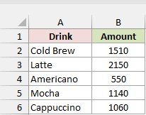
B1 contains Amount. Consolidate lists the drinks in its own order, so they may not match your summary list:
- Cold Brew: 1510
- Latte: 2150
- Americano: 550
- Mocha: 1140
- Cappuccino: 1060
These results are plain values. When the source data changes, run Consolidate again to update them. It remembers the references you added.
Note: The Consolidate dialog also has a Create links to source data option if you want to keep the output linked to its sources.
Method #6: Using Power Query
For monthly data you’ll combine repeatedly, Power Query lets you set up the append and grouping steps once, then refresh the result when needed.
Below I have the Jan sheet with ten orders, drink names, and amounts. Feb and Mar have the same layout.
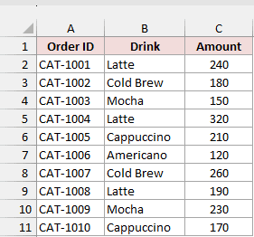
I want a table showing the combined sales for each drink. I’ll first create a query for each month, then append and group their rows.
Here are the steps to build the sales summary:
- Click inside the Jan data and press Ctrl+T. Keep My table has headers checked and click OK. On Table Design, use the Table Name box to name the table
JanSales. In newer versions of Microsoft 365, you can enterJanSalesdirectly in the Create Table dialog’s What is the name of your table? box.
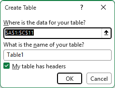
- With a cell in JanSales selected, go to Data > From Table/Range. The Power Query Editor opens with the JanSales query.
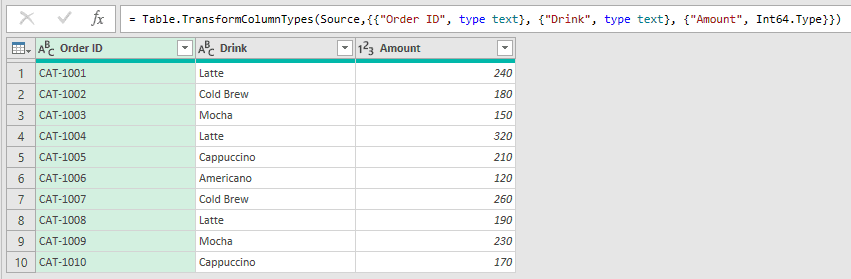
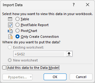
- In the editor, open the Home > Close & Load dropdown and choose Close & Load To…. Select Only Create Connection, then click OK.
- Repeat steps 1 through 3 for Feb and Mar. Name their Excel Tables
FebSalesandMarSales, and create a connection-only query for each.
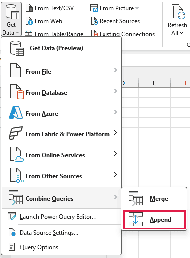
- Back in Excel, go to Data > Get Data > Combine Queries > Append.
- In the Append dialog, choose Three or more tables. Add JanSales, FebSales, and MarSales to Tables to append, in that order, then click OK.
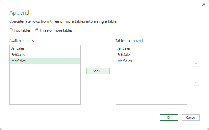
The editor opens with all 30 orders stacked in a query named Append1. Next, group those rows by drink to calculate the totals.
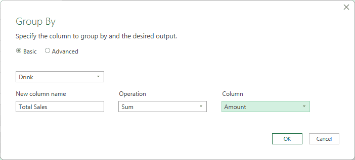
- Select the Drink column and choose Home > Group By. In the dialog’s Basic view, group by Drink, set New column name to
Total Sales, Operation to Sum, and Column to Amount. Click OK.
- Choose Home > Close & Load. Excel loads the result as a new table on a new sheet.
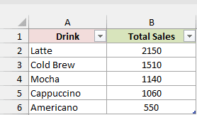
The table has Drink and Total Sales headers. Its rows follow the drinks’ order of first appearance:
- Latte: 2150
- Cold Brew: 1510
- Mocha: 1140
- Cappuccino: 1060
- Americano: 550
After changing the monthly data, use Data > Refresh All to update the summary. Power Query refresh is manual.
Note: A new month isn’t included automatically. Create its table and query, then use Home > Append Queries in the editor to add it to the append.
Additional Notes About Using SUMIF Across Multiple Sheets in Excel
Keep these details in mind when setting up your monthly sheets:
- Keep the same layout on every source sheet. These examples expect drink names in column B and amounts in column C.
- A 3D range such as
Jan:Marincludes every sheet between those tabs. Moving a sheet outside that range removes it from the calculation. - Use ranges covering the longest monthly sheet for SUMIF and FILTER; both ignore blank rows when matching drink names. If GROUPBY ranges extend past the data, blank rows form an extra group labeled 0, with a 0 total, above the Total row. Keep GROUPBY ranges to the actual data.
- Formula methods recalculate when the source data changes. Consolidate needs another run, and Power Query needs a manual refresh through Data > Refresh All.
Frequently Asked Questions
Here are a few questions people often ask about adding up values across sheets.
Why Does SUMIF With Jan:Mar! Return #VALUE!?
SUMIF doesn’t accept a 3D reference such as Jan:Mar!B2:B11.
Each SUMIF range argument must point to cells on one sheet, so a reference spanning several sheets makes it return #VALUE!.
SUMIFS, COUNTIF, and COUNTIFS have the same restriction. A function such as VSTACK can combine those sheets’ data first, which is why Method #2 works.
Can I Use SUMIFS Across Multiple Sheets?
Yes. Methods #1 and #3 can use SUMIFS in place of SUMIF when you need multiple conditions.
Check the argument order when making that change. SUMIFS takes the sum range first, while SUMIF takes its criteria range first.
With the VSTACK approach, add the second condition inside FILTER before SUM adds the matching amounts.
Will a New Sheet Be Included Automatically?
With the VSTACK formulas, yes, if you insert the new sheet between Jan and Mar. A sheet outside those boundary tabs won’t be included.
For Method #1, add another SUMIF. For Method #3, add the sheet name and extend the list range in the formula.
For Consolidate, add the new reference and run it again. For Power Query, add the month’s table and query to the append, then refresh.
Does SUMIF Work Across Different Workbooks?
SUMIF can reference another workbook, but it returns #VALUE! when that source workbook is closed. Keep the source workbook open for the calculation.
The VSTACK and INDIRECT approaches shown here are for sheets in the same workbook.
Conclusion
I’ve covered six ways to total values across sheets when SUMIF alone can’t.
I’d use VSTACK and FILTER by default in Microsoft 365 or Excel 2024.
I hope you found this article helpful.
Other Excel articles you may also like:
- SUM Function in Excel (6 Easy Examples)
- How to Add Cells in Excel (7 Easy Ways)
- How to Use SUMIFS with INDEX MATCH in Excel (6 Easy Ways)
- SUMPRODUCT vs SUMIFS Function in Excel
- SUMPRODUCT Function in Excel (5 Easy Examples)
- SUMIF vs SUMIFS Function in Excel (7 Clear Examples)
- How to Reference a Cell on Another Sheet in Excel
- How to VLOOKUP Between Two Sheets in Excel (4 Easy Ways)
