
An aging report sorts unpaid invoices by how many days they are past due. It shows which balances are current and which ones need attention.
Excel can calculate the late days and assign each invoice to a Current, 1-30, 31-60, 61-90, or 90+ day bucket.
I’ll use a fixed as-of date, so the report stays unchanged when you save or send it. A live report can use TODAY() instead.
Calculate the Days Past Due First
Before assigning aging buckets, calculate how late each invoice is. Use the Due Date because it already accounts for the customer’s payment terms.
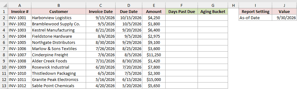
Below I have a dataset of 12 unpaid invoices with their invoice dates, due dates, amounts, and a fixed As-of Date of September 30, 2026.
Enter this formula in cell F2 on the Aging Report sheet:
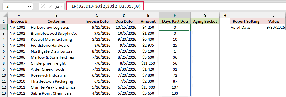
=IF(D2:D13<$J$2,$J$2-D2:D13,0)
How does this formula work?
The formula compares every Due Date in D2:D13 with the As-of Date in J2. For overdue invoices, it subtracts the Due Date from that fixed date.
Invoices that are not yet due return 0 instead of a negative number. The formula spills all 12 results down column F automatically.
A fixed date keeps a saved report reproducible. If you want the aging to move forward each day, replace $J$2 with TODAY().
This formula spills in Excel 2021, Excel 2024, and Microsoft 365. In Excel 2019 or older, enter =IF(D2<$J$2,$J$2-D2,0) in F2 and fill it down through row 13.
Method #1: Using XLOOKUP With a Bucket Table
This is the method I recommend for most readers. You can change an aging boundary or label by editing the bucket table instead of rebuilding the formula.
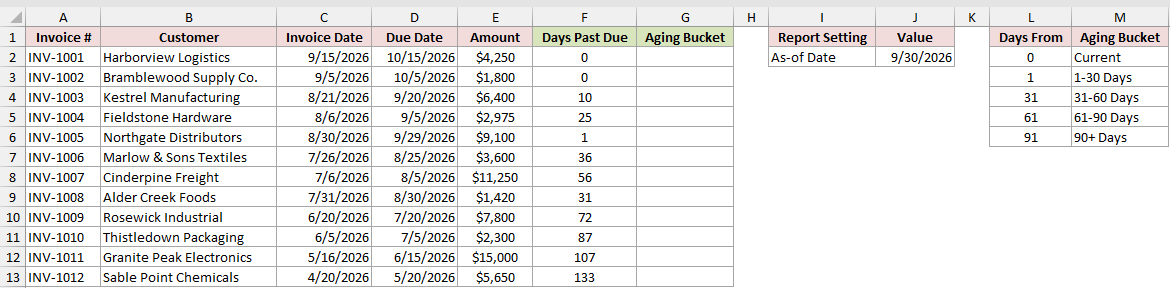
Below I have a dataset with the calculated Days Past Due column and a five-row bucket table containing each lower boundary and its Aging Bucket label.
Enter this formula in cell G2:
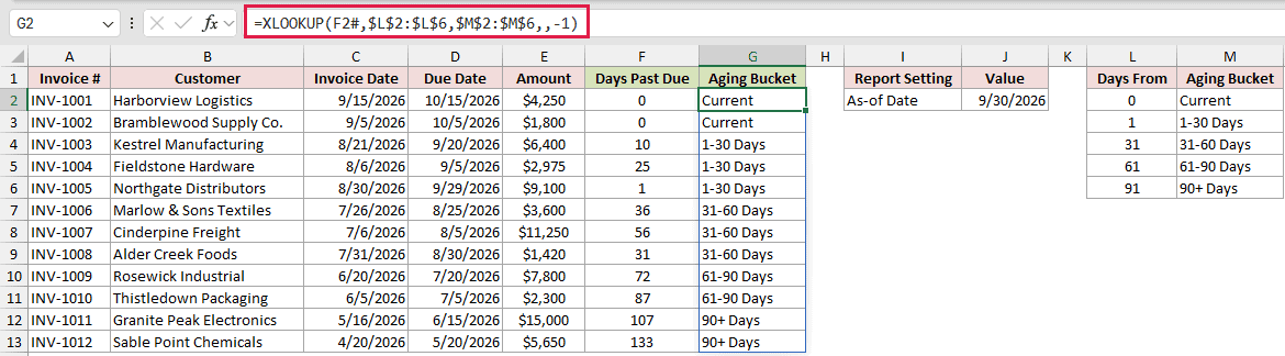
=XLOOKUP(F2#,$L$2:$L$6,$M$2:$M$6,,-1)
How does this formula work?
F2# refers to the entire spilled Days Past Due range. XLOOKUP searches for each value in the lower boundaries stored in L2:L6.
The -1 match mode returns an exact match or the next smaller boundary. A value of 36 therefore matches 31 and returns 31-60 Days.
The formula spills the Aging Bucket results down column G. In this example, the 12 invoices are distributed across all five buckets.
Note: XLOOKUP is available in Microsoft 365 and Excel 2021 or later. Use the nested IF or VLOOKUP method in an older version.
Method #2: Using Nested IF Functions
If you prefer to keep the bucket rules inside one formula, nested IF functions are a straightforward option.
Below I have a dataset of 12 invoices with Days Past Due already calculated in column F. Column G is ready for the five aging labels.
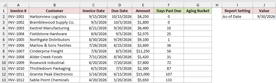
Enter this formula in cell G2 on the Nested IF sheet:
=IF(F2:F13=0,"Current",IF(F2:F13<=30,"1-30 Days",IF(F2:F13<=60,"31-60 Days",IF(F2:F13<=90,"61-90 Days","90+ Days"))))
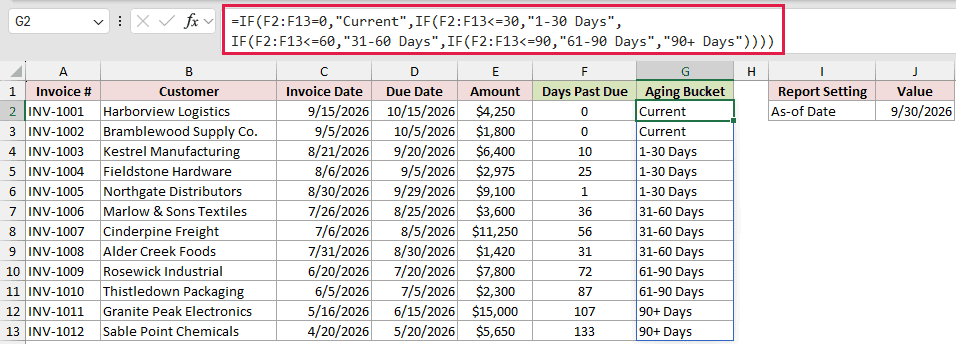
How does this formula work?
The first IF assigns Current when Days Past Due equals 0. Each later IF checks the next upper boundary: 30, 60, and 90 days.
Anything above 90 reaches the final result, 90+ Days. The range reference makes all 12 bucket labels spill from G2.
In Excel 2019 or older, use single-cell references for row 2, then fill the days and bucket formulas down the columns.
Method #3: Using VLOOKUP With Approximate Match
For an aging formula that works in every Excel version, use VLOOKUP with the same lower-bound bucket table.
Below I have a dataset of 12 unpaid invoices, the fixed As-of Date, and a bucket table sorted from the smallest Days From value to the largest.
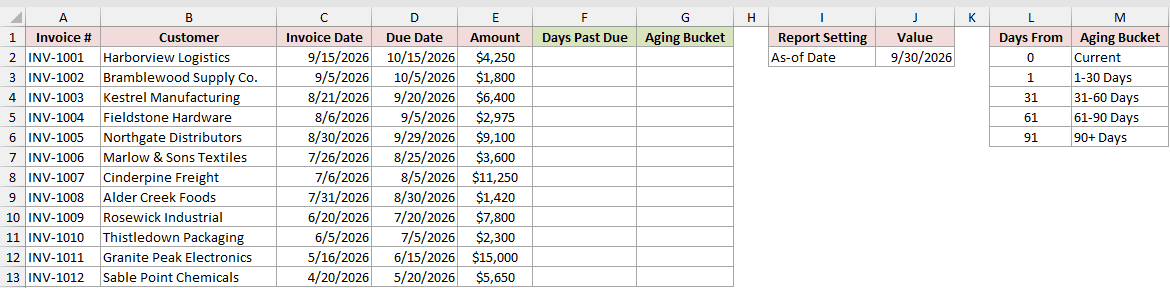
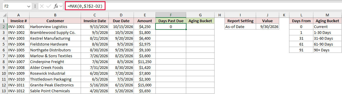
Enter this formula in cell F2 on the VLOOKUP sheet to calculate Days Past Due for the first invoice:
=MAX(0,$J$2-D2)
Then enter this formula in cell G2:
=VLOOKUP(F2,$L$2:$M$6,2,TRUE)
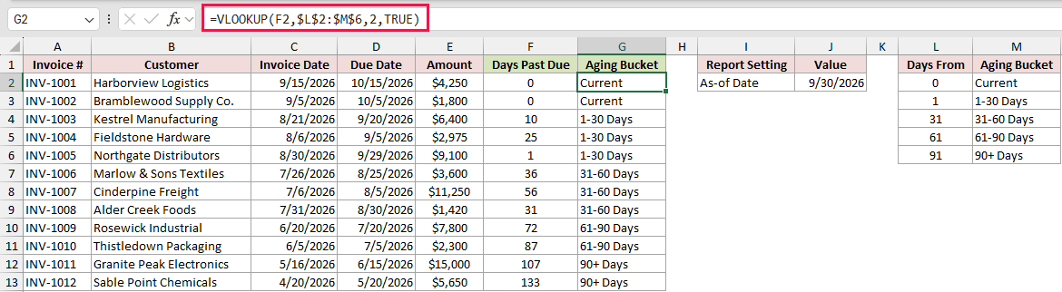
Fill both formulas down through row 13.
How does this formula work?
MAX compares 0 with the difference between the As-of Date and Due Date. It keeps future-due invoices at 0 instead of returning negative days.
VLOOKUP searches the first column of L2:M6. The column index 2 tells Excel to return the corresponding Aging Bucket from the second column.
TRUE requests an approximate match. Excel finds the largest lower boundary that does not exceed the Days Past Due value.
Create an Aging Summary by Bucket
Once the invoices have aging labels, you can see the whole accounts receivable position in a compact summary.
Below I have a dataset on the Aging Summary sheet with the five Aging Bucket labels in A2:A6 and columns for invoice counts and amounts due.
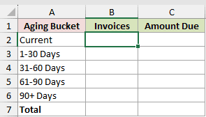
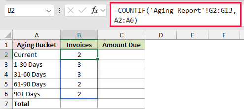
Enter this formula in cell B2 to count the invoices in each bucket:
=COUNTIF('Aging Report'!G2:G13,A2:A6)
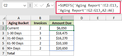
Enter this formula in cell C2 to total the outstanding amounts:
=SUMIFS('Aging Report'!E2:E13,'Aging Report'!G2:G13,A2:A6)
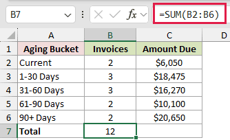
Use this formula in B7 for the total invoice count:
=SUM(B2:B6)
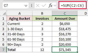
Use this formula in C7 for the total amount due:
=SUM(C2:C6)
How does this formula work?
COUNTIF compares the Aging Report labels with all five labels in A2:A6. It spills one invoice count for each bucket.
SUMIFS uses those same labels as criteria and adds the matching invoice amounts. It also spills five results down the Amount Due column.
The summary returns 2 Current invoices worth $6,050 and 3 invoices in 1-30 Days worth $18,475.
Rows for 31-60, 61-90, and 90+ Days show 3 at $16,270, 2 at $10,100, and 2 at $20,650.
The total row confirms that the report contains 12 invoices with $71,545 outstanding.
In Excel 2019 or older, reference a single label such as A2 in both formulas, then fill B2 and C2 down through row 6.
Additional Notes About Aging Formulas in Excel
- Calculate aging from the Due Date, not the Invoice Date. The Due Date already includes agreed payment terms such as Net 30.
- Fill missing Due Dates or guard them with an IF test. Excel treats a blank date as zero, which can create a huge false overdue value.
- Remove paid invoices or filter them out before aging the list. Otherwise, settled balances will still appear in the report.
- Keep lookup-table boundaries sorted from smallest to largest. Incorrect sorting can make an approximate-match formula return the wrong bucket without an error.
Frequently Asked Questions
How Do I Age Invoices From the Invoice Date Instead?
Replace the Due Date reference with the Invoice Date reference in the Days Past Due formula. This measures age from issue rather than lateness after payment terms.
How Do I Make an Aging Report Update Every Day?
Replace the fixed As-of Date reference, $J$2, with TODAY(). Excel will recalculate the aging whenever the workbook recalculates on a new date.
Can I Use a PivotTable for an Aging Summary?
Yes. Put Aging Bucket in the Rows area and Amount in Values, summarized by Sum. Refresh the PivotTable when the source data changes.
How Do I Add a 120+ Day Bucket?
For XLOOKUP or VLOOKUP, relabel the 91 row 91-120 Days and add a 121 row labeled 120+ Days.
For nested IF, add another test for values at or below 120 before the final 120+ Days result.
Conclusion
These formulas calculate Days Past Due, assign every invoice to a 30, 60, or 90-day aging bucket, and summarize the outstanding balance.
I recommend XLOOKUP with a bucket table because changing a boundary takes one table edit. Nested IF and VLOOKUP remain reliable choices for older Excel versions.
I hope you found this article helpful!
Other Excel articles you may also like:
