How to Use IF With Cell Color in Excel

Excel’s IF function can’t look at a cell’s fill color. It only reads values, so a formula like =IF(A2 is green,…) doesn’t exist out of the box.

That’s a problem when someone has marked rows by coloring them. The color carries the meaning, but none of your formulas can see it.

There are workarounds, though. You can read the color with an old macro function or a short piece of VBA, then feed that into IF.

In this article, I’ll show you how to use IF with GET.CELL and a custom VBA function, fill in values with Filter by Color, and color cells based on an IF result.

Method #1: Using GET.CELL in a Named Range (Recommended)

GET.CELL is an old Excel 4.0 macro function that can return a cell’s fill color. It doesn’t work in a cell directly, but it works fine inside a defined name.

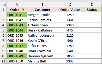
Below I have a dataset of orders. The Order ID cells of shipped orders are filled green.

I want the Status column to say Shipped or Pending based on that color.

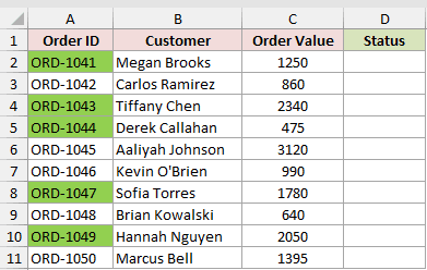
Here are the steps to create the named range:

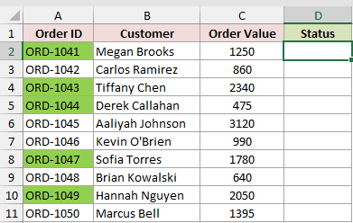
1. Select cell D2. The name uses a relative reference, so the active cell matters here.

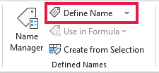
2. On the Formulas tab, click Define Name.

3. In the New Name dialog box, type CellColor in the Name field and enter =GET.CELL(38,Orders!$A2) in the Refers to field. Then click OK.

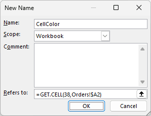
The 38 tells GET.CELL to return the fill color of the cell.

The $A2 reference locks the column but not the row, so the name always checks column A in the same row as your formula.

Before writing the IF formula, you need the number Excel uses for your green.

Enter =CellColor in any cell in row 2 and it returns 43. A cell with no fill returns 0.

Now enter this formula in cell D2:

=IF(CellColor=43,"Shipped","Pending")

Then copy it down to D11.

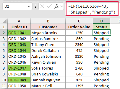
How does this formula work?

CellColor returns the color number of the Order ID cell in the same row. For the green cells, that number is 43.

IF then checks whether the number equals 43. If it does, the formula returns Shipped. If not, it returns Pending.

Note: GET.CELL counts as a macro function, so save the file as an Excel Macro-Enabled Workbook (.xlsm). If you try to save it as a regular .xlsx file, Excel warns you that it can’t keep the macro content in a macro-free workbook.

Method #2: Using a Custom VBA Function

If you’re fine with a bit of VBA, you can write your own function that checks the color.

Once it’s in the workbook, you use it inside IF like any other function.

Below I have the same orders dataset. The shipped orders have a green Order ID, and I want Shipped or Pending in the Status column.

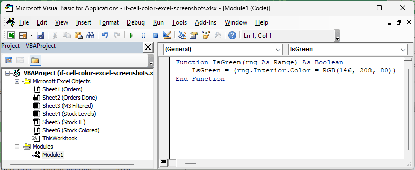
Here is the VBA code:

Function IsGreen(rng As Range) As Boolean
    IsGreen = (rng.Interior.Color = RGB(146, 208, 80))
End Function

Function IsGreen(rng As Range) As Boolean
    IsGreen = (rng.Interior.Color = RGB(146, 208, 80))
End Function

Here are the steps to add this function:

1. Press Alt + F11 to open the VBA Editor.
2. Click Insert, then Module.
3. Paste the code above into the module window.

4. Close the VBA Editor and go back to the worksheet.

Now enter this formula in cell D2 and copy it down to D11:

=IF(IsGreen(A2),"Shipped","Pending")

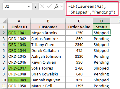
How does this formula work?

IsGreen looks at the fill color of the cell you give it.

It returns TRUE when the color is RGB(146, 208, 80), which is the Light Green swatch under Standard Colors, and FALSE otherwise.

IF then returns Shipped for TRUE and Pending for FALSE.

If your cells use a different color, change the RGB values in the code. You can get them from Home, Fill Color, More Colors, on the Custom tab.

Note: Save the file as an Excel Macro-Enabled Workbook (.xlsm) to keep the function. In a regular .xlsx file, the code is removed and the formulas return #NAME?.

Method #3: Using Filter by Color

If you don’t need a live formula and only want to fill in the Status column once, Filter by Color does it without any code.

Below I have the orders dataset again. The green Order IDs are the shipped orders, and I want to type Shipped or Pending in column D.

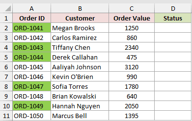
Here are the steps:

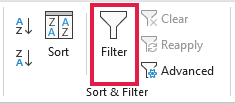
1. Select any cell in the dataset, and on the Data tab, click Filter.

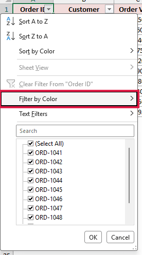
2. Click the filter arrow in the Order ID header, point to Filter by Color, and pick the green color.

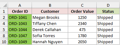
3. Select the Status cells of the visible rows, press Alt + ; so only visible cells stay selected, type Shipped, and press Ctrl + Enter.

4. Open the Order ID filter again, point to Filter by Color, and pick No Fill. Then repeat step 3, typing Pending this time.
5. On the Data tab, click Filter again to remove the filter.

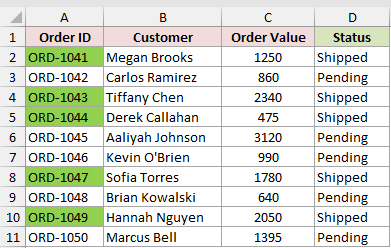
The Status column now says Shipped for the five green orders and Pending for the other five.

These are typed values, not formulas. If you recolor a cell later, the status doesn’t change, so you’d have to repeat the steps.

Method #4: Using IF With Conditional Formatting

Sometimes the question is the other way around. You want a cell to turn a color based on what an IF formula returns, and that part Excel handles natively.

Below I have a dataset of products and how many units are in stock.

I want an Action column that says Reorder when stock is under 20, and I want those cells highlighted.

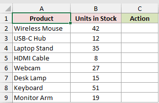
First, enter this formula in cell C2 and copy it down to C9:

=IF(B2<20,"Reorder","OK")

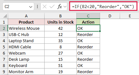
The formula returns Reorder for USB-C Hub, HDMI Cable, Desk Lamp, and Monitor Arm, since those have fewer than 20 units. Everything else shows OK.

Here are the steps to color the Reorder cells:

1. Select C2:C9.
2. On the Home tab, click Conditional Formatting, then New Rule.

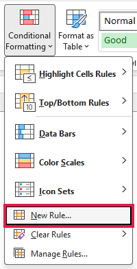
3. Choose “Use a formula to determine which cells to format” and enter =$C2=”Reorder” in the formula box.
4. Click Format, pick a fill color on the Fill tab, and click OK twice.

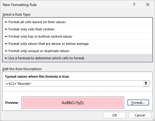
The four Reorder cells are now filled with the color you picked.

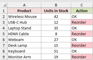
Because the rule checks the formula’s result, the color updates by itself.

If you change Webcam’s stock to 10, its Action changes to Reorder and the cell gets colored right away.

Note: You don’t need the IF column for this. A rule of =$B2<20 applied to the data colors the same rows directly. The IF column is useful when you also want the Reorder label in the sheet.

Additional Notes About Using IF With Cell Color in Excel

• Changing a color doesn’t recalculate the formula. Recoloring a cell isn’t an edit, so GET.CELL and the VBA function keep the old result. Even F9 doesn’t help. Press Ctrl + Alt + F9 to force a full recalculation.
• Conditional formatting colors can’t be read. GET.CELL returns 0 for a cell colored by a conditional formatting rule. In that case, use the rule’s own condition in your IF formula instead.
• GET.CELL returns a palette number, not an exact color. It uses Excel’s 56-color index, so two similar shades can return the same number. The VBA function compares the exact RGB color, so it doesn’t have this problem.
• Both formula methods need a macro-enabled file. Save as .xlsm, and enable macros when you reopen the file, or the formulas stop working.
• The shortcuts here are the Windows ones. On a Mac, press Option + F11 for the VBA Editor and Ctrl + Option + F9 to force a recalculation. Ctrl + Enter works the same on both. There is no Mac equivalent of Alt + ;, so pick visible cells from Home, Find & Select, Go To Special, Visible cells only.

Frequently Asked Questions

Can I Use IF With Cell Color Without VBA?

Yes. Method #1 uses GET.CELL inside a named range, which needs no VBA code.

The file still has to be saved as .xlsm, though, because GET.CELL is treated as a macro function.

How Do I Find the Color Number of a Cell?

Create the CellColor name from Method #1 and enter =CellColor in a cell on the same row.

It returns the color index of the cell in column A. A cell with no fill returns 0.

Can I Sum Values Based on Cell Color?

Yes. Filter the column by color as in Method #3, then use =SUBTOTAL(9,C2:C11). SUBTOTAL ignores rows hidden by a filter, so it sums only the visible, colored rows.

Why Does My Color Formula Return #NAME?

The workbook was probably saved as .xlsx, or macros are disabled. Reopen the .xlsm version and click Enable Content in the yellow security bar.

Conclusion

In this article, I showed you how to use IF with cell color through GET.CELL in a named range, a custom VBA function, Filter by Color, and conditional formatting.

I reach for GET.CELL first, since it reads the color without any code. I hope you found this article helpful.

Other Excel articles you may also like:

• Count Colored Cells in Excel
• Change Cell Color Based on Text Input in Excel
• How to Change Cell Color Using VBA in Excel
• Change Cell Color Based on Value of Another Cell in Excel
• How to Change Font Color Based on Cell Value in Excel?
• Highlight Cell If Value Exists in Another Column in Excel
• Create a Drop-down List with Color in Excel