
To calculate a percentile with criteria in Excel, pick the rows that meet your conditions and pass their numbers to PERCENTILE.INC. That gives you a cutoff for the group you care about, such as the 90th percentile delivery time for orders from one warehouse.
I’ll show you how to do this for one condition or several, what to use in older Excel, and how to get a percentile for every group in one report.
Method #1: Using PERCENTILE.INC With FILTER
This is the formula I’d use in Microsoft 365, Excel 2024, or Excel 2021. FILTER picks out the numbers you want, and PERCENTILE.INC calculates the cutoff from those numbers.
On the Criteria sheet, I have 18 laundromat loads. Column B has the fabric, column C has the cycle, and column D has the drying time in minutes. The settings in G2:G4 are Cotton, Standard, and 0.75.
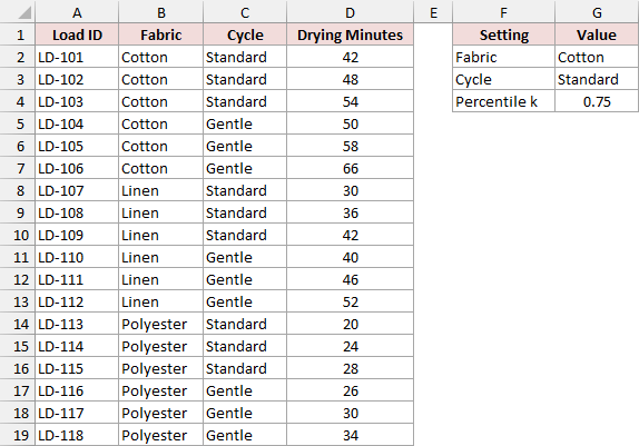
Calculate a Percentile With One Criterion
To find the 75th percentile for cotton loads across both cycles, enter this formula in F7.
=PERCENTILE.INC(FILTER($D$2:$D$19,($B$2:$B$19=$G$2)*ISNUMBER($D$2:$D$19)),$G$4)
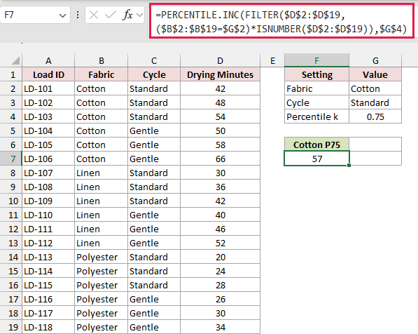
The result is 57 minutes. The test on column B keeps Cotton, and ISNUMBER makes sure the matching time is a number. FILTER passes those six times to PERCENTILE.INC, which uses 0.75 from G4.
The two times around the cutoff are 54 and 58 minutes. Excel interpolates between them, so the answer can fall between recorded times.
Calculate a Percentile With AND Criteria
Now suppose you only want cotton loads that ran on the Standard cycle. Enter this formula in G7.
=PERCENTILE.INC(FILTER($D$2:$D$19,($B$2:$B$19=$G$2)*($C$2:$C$19=$G$3)*ISNUMBER($D$2:$D$19)),$G$4)
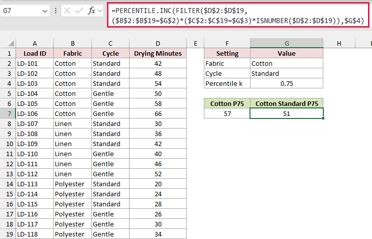
The result is 51 minutes. Multiplying the tests works like AND. A row makes it through only when the fabric is Cotton, the cycle is Standard, and the drying time is numeric. That leaves 42, 48, and 54 minutes.
Calculate a Percentile With OR Criteria
To include either cotton or linen, enter this formula in H7. This example includes both cycles.
=PERCENTILE.INC(FILTER($D$2:$D$19,((($B$2:$B$19=$G$2)+($B$2:$B$19="Linen"))>0)*ISNUMBER($D$2:$D$19)),$G$4)
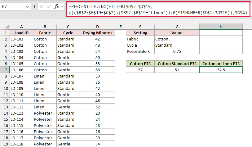
The result is 52.5 minutes. Adding the two fabric tests and checking for a sum greater than zero means either test can pass. The numeric check still applies to every row.
Note: Enter 0.75 or 75% for the 75th percentile. Entering 75 by itself is outside the range PERCENTILE.INC accepts.
Method #2: Using PERCENTILE.INC With IF
If you’re working in Excel 2016 or 2019, you can use IF to select the drying times. In this example, I want the 75th percentile for the Cotton loads that ran on Standard. The fabric, cycle, and percentile are in G2:G4 on the Criteria sheet.
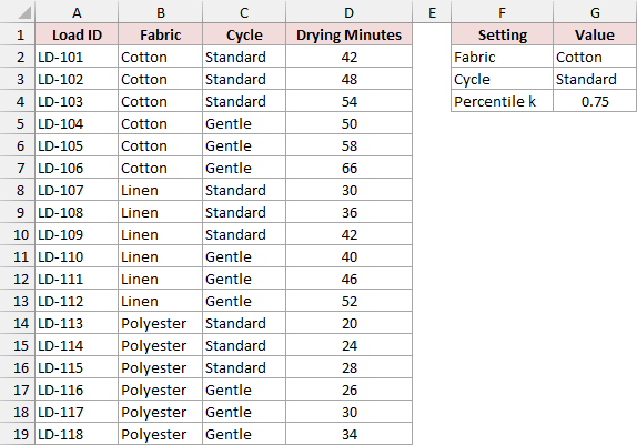
Use this formula in an empty cell. In Excel 2016 or 2019, confirm it with Ctrl+Shift+Enter on Windows. In current Excel with dynamic arrays, press Enter.
=PERCENTILE.INC(IF(($B$2:$B$19=$G$2)*($C$2:$C$19=$G$3)*ISNUMBER($D$2:$D$19),$D$2:$D$19),$G$4)
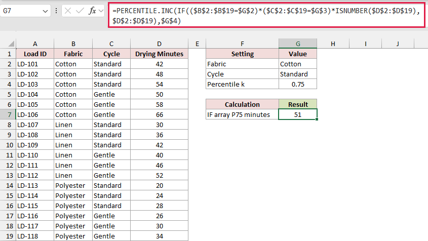
IF returns the drying time for each qualifying row and FALSE for the others. PERCENTILE.INC skips those FALSE values and returns 51 minutes.
If you use Ctrl+Shift+Enter, Excel adds braces around the formula in the formula bar.
Method #3: Using the AGGREGATE Function
AGGREGATE is handy in older Excel if you want to enter the formula with Enter. On the Criteria sheet, I’m using the fabric and cycle in G2 and G3 to find the 75th percentile drying time for cotton on Standard.
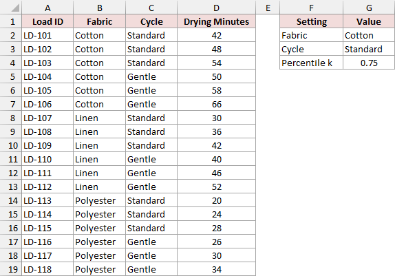
Enter this formula in an empty cell and press Enter.
=AGGREGATE(16,6,$D$2:$D$19/(($B$2:$B$19=$G$2)*($C$2:$C$19=$G$3)*ISNUMBER($D$2:$D$19)),$G$4)
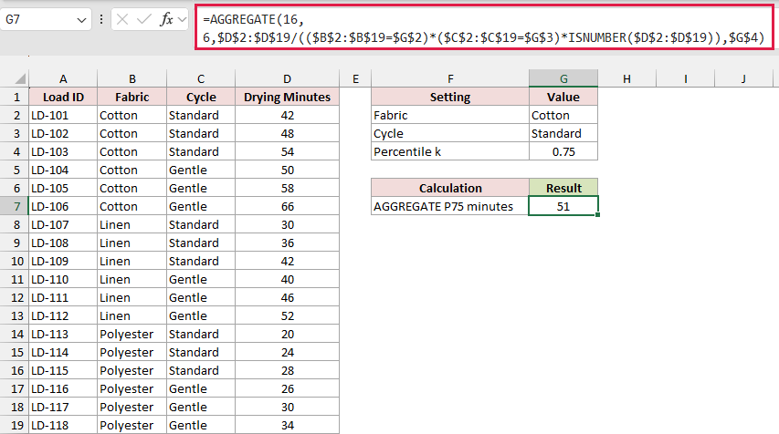
The result is 51 minutes. The first argument, 16, tells AGGREGATE to calculate an inclusive percentile. The second argument, 6, tells it to skip errors.
For a row that meets all three tests, the formula divides the drying time by 1 and keeps the original number. Rows that fail the tests produce errors. AGGREGATE skips those rows and calculates the percentile of the remaining values.
The same option also skips errors that already exist in the source. If a drying time contains an error you need to investigate, check the source before relying on the result.
Method #4: Using GROUPBY With LAMBDA
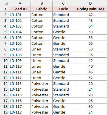
Use GROUPBY if you want all the cutoffs at once. On the Grouped Formula sheet, columns B and C contain the fabric and cycle for each load, and column D contains its drying time.
I want one 75th percentile for each fabric and cycle combination.
In Microsoft 365 with GROUPBY available, enter this formula in F2.
=GROUPBY(B2:C19,D2:D19,LAMBDA(v,PERCENTILE.INC(v,0.75)),0,0)
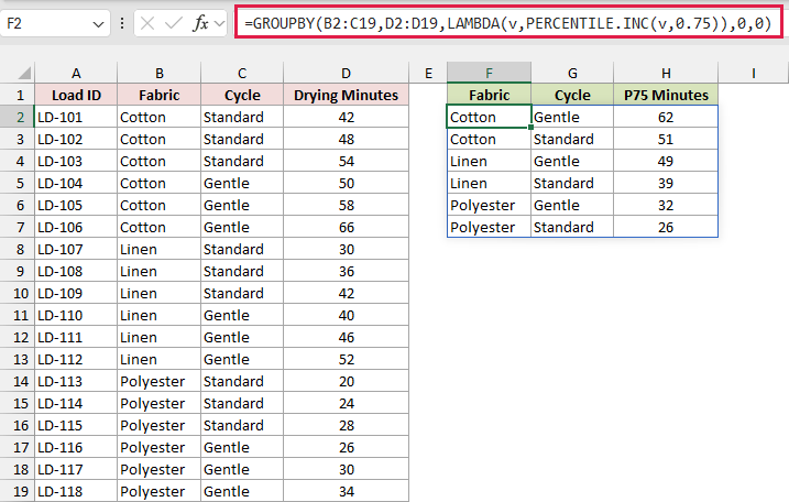
The results spill into F2:H7. For example, Cotton on Gentle comes out at 62 minutes, and Cotton on Standard comes out at 51 minutes.
GROUPBY groups the rows by the two columns in B2:C19. LAMBDA gives GROUPBY a calculation to run for each group. Its v holds that group’s drying times, and PERCENTILE.INC gets their 75th percentile.
The first 0 tells GROUPBY that the inputs exclude headers and that it should return just the results. The second 0 turns off totals. The headers above the formula in the example are already typed in.
Method #5: Grouping Rows in Power Query
I use Power Query when I want to keep the same report and refresh it after adding new records.
The Power Query sheet has the load data in A1:D19. I’ll use the fabric and cycle to calculate a separate 75th percentile for each combination.
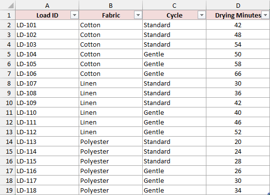
The example already has a working query. To build it yourself, copy the source data into a blank workbook and follow these steps in desktop Excel for Windows.
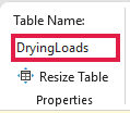
- Select the source data and press Ctrl+T. Check My table has headers, then click OK. On the Table Design tab, set Table Name to
DryingLoads.
- Select a cell in the table and choose Data > From Table/Range to open the Power Query Editor.
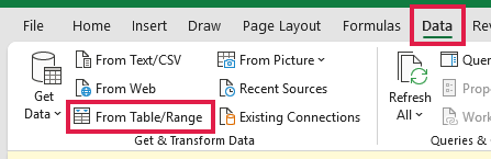
- In the Power Query Editor, choose Home > Advanced Editor. Replace the existing code with the code below and click Done.
let
    Source = Excel.CurrentWorkbook(){[Name="DryingLoads"]}[Content],
    NumericLoads = Table.SelectRows(Source,each Value.Is([Drying Minutes],type number)),
    Grouped = Table.Group(NumericLoads,{"Fabric","Cycle"},{{"P75 Minutes",each List.Percentile([Drying Minutes],0.75,[PercentileMode=PercentileMode.ExcelInc]),type number}}),
    Sorted = Table.Sort(Grouped,{{"Fabric",Order.Ascending},{"Cycle",Order.Ascending}})
in
    Sorted

- Choose Home > Close & Load to load the summary as a table on a new worksheet.
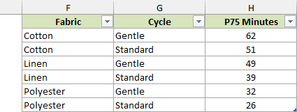
The query reads the named Excel table and keeps rows with numeric drying times. It groups by Fabric and Cycle and uses List.Percentile on the times in each group. The ExcelInc setting uses the same interpolation as PERCENTILE.INC.
The finished sample places the loaded table beside the source data so you can compare them. It returns six rows, including 51 minutes for Cotton on Standard. After adding rows to the source table, choose Data > Refresh All to update the report.
Additional Notes About Calculating Percentiles With Criteria in Excel
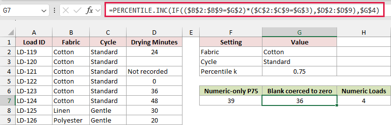
Check which rows go into the calculation when a percentile looks off. On the Data Checks sheet, Cotton on Standard includes a blank, a text entry, and a recorded zero alongside the other times.
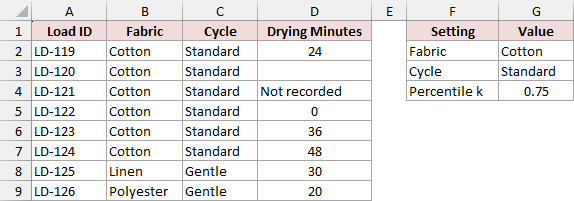
The numeric-only formula in F7 uses four times (0, 24, 36, and 48 minutes). The 75th percentile is 39 minutes.
=PERCENTILE.INC(FILTER($D$2:$D$9,($B$2:$B$9=$G$2)*($C$2:$C$9=$G$3)*ISNUMBER($D$2:$D$9)),$G$4)
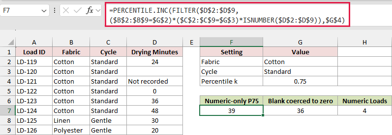
The comparison in G7 drops the numeric test. Here, IF turns the matching blank into a second zero, which moves the percentile down to 36 minutes.
=PERCENTILE.INC(IF(($B$2:$B$9=$G$2)*($C$2:$C$9=$G$3),$D$2:$D$9),$G$4)
Frequently Asked Questions
Here are a few checks that come up when you use these formulas on your own data.
Does Excel Have a PERCENTILEIF or PERCENTILEIFS Function?
Excel has neither function built in. You can use PERCENTILE.INC with FILTER to select the values that meet your conditions, then calculate the percentile from those values.
Do Hidden or Filtered-Out Rows Count?
Yes, if they match the criteria in the worksheet formulas above. Hiding a row or applying a filter from the Data tab leaves that row in the referenced range. The formulas check the cell values directly.
What Happens When No Numeric Rows Match?
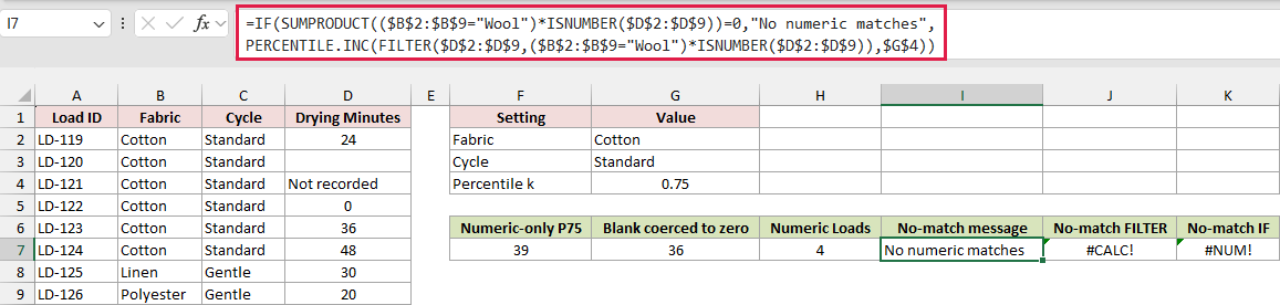
On Data Checks, a search for Wool has no matches. The FILTER version in J7 returns #CALC! because the filtered array is empty. The IF version in K7 returns #NUM! because there are no numbers for PERCENTILE.INC.
To return a message instead, count the matching numeric rows before calculating the percentile. Here’s the formula in I7.
=IF(SUMPRODUCT(($B$2:$B$9="Wool")*ISNUMBER($D$2:$D$9))=0,"No numeric matches",PERCENTILE.INC(FILTER($D$2:$D$9,($B$2:$B$9="Wool")*ISNUMBER($D$2:$D$9)),$G$4))
Should I Use PERCENTILE.INC or PERCENTILE.EXC?
I use PERCENTILE.INC unless a reporting requirement calls for the exclusive calculation. PERCENTILE.INC accepts percentiles from 0% through 100%. PERCENTILE.EXC uses different interpolation and can return #NUM! near the ends when the group is small.
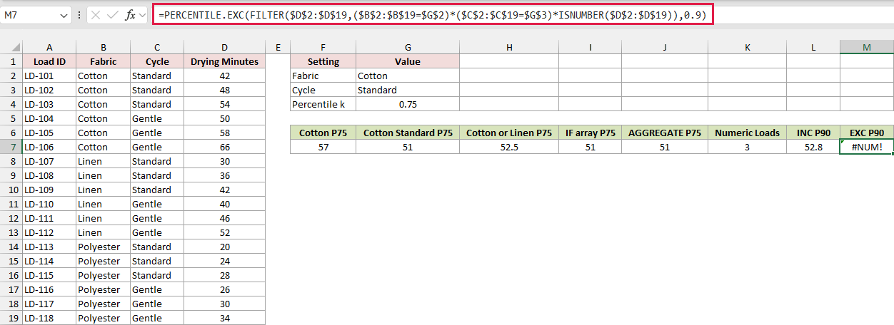
On Criteria, only three rows match Cotton and Standard. At the 90th percentile, PERCENTILE.INC gives 52.8 minutes in L7, and the exclusive calculation in M7 gives #NUM!.
=PERCENTILE.EXC(FILTER($D$2:$D$19,($B$2:$B$19=$G$2)*($C$2:$C$19=$G$3)*ISNUMBER($D$2:$D$19)),0.9)
Conclusion
In this article, I showed you how to calculate percentiles with one or more criteria, handle blanks and missing matches, and build grouped summaries. I hope you found this article helpful.
Other Excel articles you may also like: