How to Sort Alphabetically in Excel

If you have a column of names, products, or any text and you want it in A-to-Z order, Excel gives you more than one way to get there.

The tricky part is doing it without scrambling the other columns that belong with each row.

The good news is that every built-in method handles that for you once you set it up right.

Below I’ll walk through six ways to sort alphabetically, from a one-click button to a formula that leaves your original data untouched.

Method #1: Using the Sort A to Z Button

The fastest way to sort alphabetically in Excel is the A to Z button on the Data tab.

Click one cell in the column you want sorted, and Excel sorts the connected data range, often called the current region, around that cell.

Below I have a menu list with the dish name, its category, and its calorie count. I want the rows sorted alphabetically by the dish name.

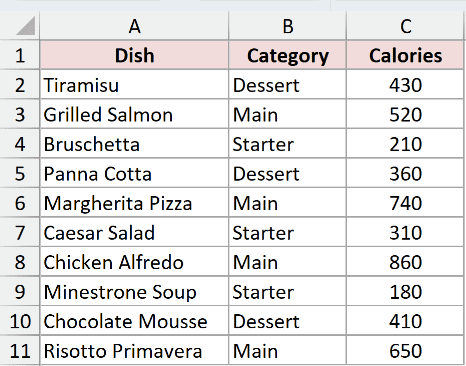
Here are the steps to sort this list alphabetically with the A to Z button:

1. Click any single cell inside the Dish column (say, cell A2).

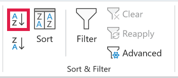
2. Go to the Data tab and, in the Sort & Filter group, click the A to Z button.

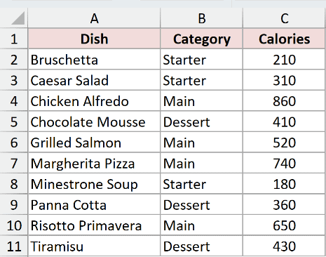
Excel sorts the whole table by dish name, so Bruschetta lands on top and Tiramisu drops to the bottom.

Each dish keeps its own category and calorie value because Excel moves the entire row, not just the one column.

Note: Click one cell inside the connected data range, not the worksheet’s entire column. If Excel shows a Sort Warning, choose Expand the selection so every cell in each row moves with its dish. Continue with the current selection can separate related cells.

Method #2: Using the Sort Dialog Box

The Sort dialog box lets you sort alphabetically by more than one column at a time.

You can group the list by category first and then sort the dishes A to Z inside each group.

Here again is the menu list with the dish, its category, and its calorie count.

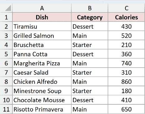
Here are the steps to sort alphabetically using the Sort dialog box:

1. Click any cell inside the data.

2. On the Data tab, click Sort to open the Sort dialog box.

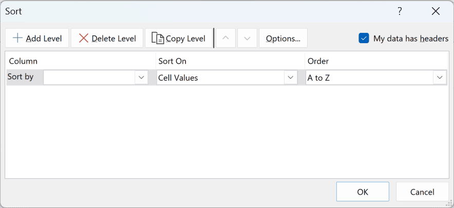
3. In the Sort by dropdown, pick Category, and leave Order set to A to Z.

4. Click Add Level, then in the Then by dropdown pick Dish, with Order set to A to Z.

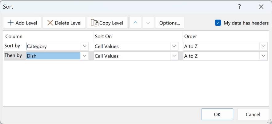
5. Click OK.

Excel now sorts the categories alphabetically first, then sorts the dishes A to Z within each category.

So all the Dessert rows sit together in A-to-Z order, then the Main rows, then the Starter rows.

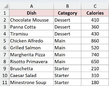
Note: Make sure the “My data has headers” box is checked in the top-right of the dialog. That keeps your header row (Dish, Category, Calories) pinned at the top instead of getting sorted into the data.

Method #3: Using the Filter Dropdown

Here’s another way to do this.

If your data already has filter buttons turned on, each column header has a dropdown with a Sort A to Z option built right in.

This is handy when you’re already filtering and just want to reorder what’s showing.

Below is the same menu list with the dish, category, and calories.

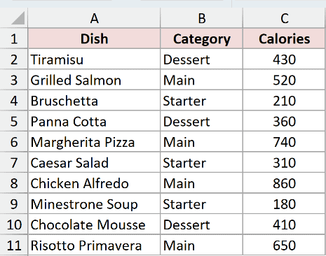
Here are the steps to sort alphabetically from the filter dropdown:

1. Click any cell in the data. In Windows, press Ctrl + Shift + L, or choose Data > Filter, to turn on the header dropdowns.

2. Click the dropdown arrow on the Dish header, then choose Sort A to Z.

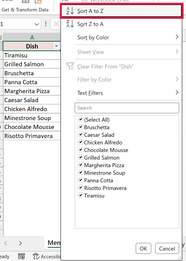
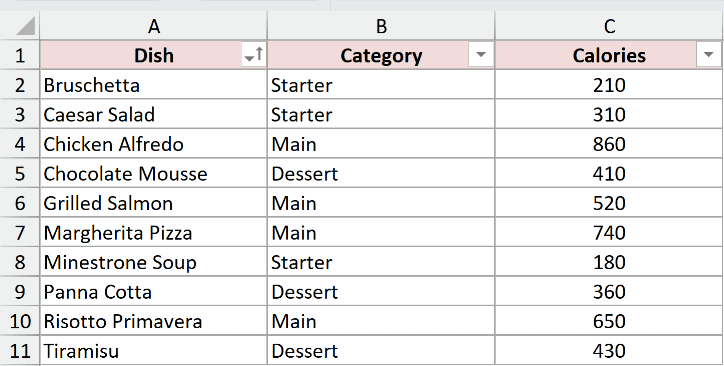
Excel sorts the full table by dish name, exactly like the A to Z button does.

A small up arrow on the Dish dropdown shows which column is sorted.

Method #4: Using the SORT Function

The SORT function gives you a sorted copy that updates when the source values change. Your original data stays where it is.

It’s a dynamic array function available in Excel for Microsoft 365 and Excel 2021 onwards.

Below I have the menu list in columns A to C, and I want a sorted-by-dish copy of the whole table to spill out in a separate spot.

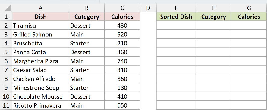
On the SORT by Dish worksheet, enter this formula in cell E2:

=SORT(A2:C11)

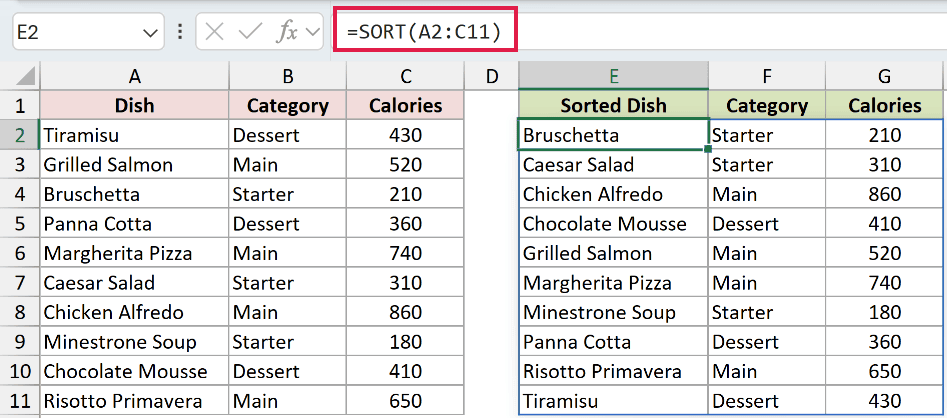
The formula spills across three columns and down ten rows automatically, sorting every dish while carrying its category and calories along.

How does this formula work?

SORT takes the range you hand it and returns a sorted copy. I gave it A2:C11, which is the whole three-column table.

I didn’t type the other arguments, so SORT falls back to its defaults.

It sorts by the first column (sort_index of 1) in ascending, A-to-Z order (sort_order of 1).

That’s exactly the alphabetical sort I wanted.

If I wanted to sort by the Category column instead, I’d write =SORT(A2:C11,2) to point it at the second column.

Because this is a live formula, editing a dish in the source range refreshes the sorted list on its own.

To include newly added rows, convert the source to an Excel Table and use a structured reference, or expand the fixed A2:C11 reference.

Note: The spilled result is a formula, so you can’t manually rearrange rows inside it. If you need to sort just the names and nothing else, point SORT at a single column with =SORT(A2:A11).

Method #5: Using Power Query

For a repeatable sort that you can rerun whenever the data changes, Power Query is a solid choice.

You sort the column once inside the query editor, load the result to a new table, and refresh it later with a click.

This suits data you pull in and clean on a regular basis.

The steps and screenshots below are for Excel on Windows.

Microsoft 365 for Mac includes Power Query under Data > Get Data, but Microsoft’s current support matrix lists Table/Range as refresh-only on Mac.

Build this exact Table/Range query in Windows, then you can refresh it on Mac.

Excel for the web can refresh supported Power Query sources, including Table/Range, subject to its refresh limits. Use desktop Excel for Windows to follow the query-editor steps below.

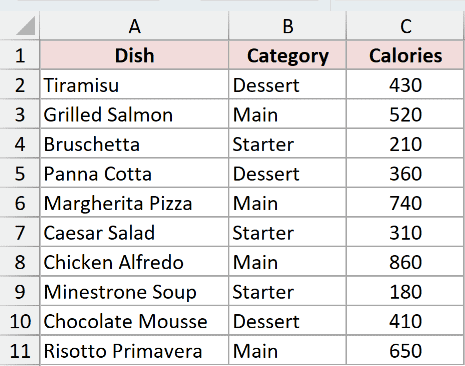
Below is the menu list I want to load into Power Query and sort alphabetically by dish.

Here are the steps to sort alphabetically using Power Query:

1. Click any cell in the data and press Ctrl + T to convert the range into an Excel Table, then click OK.

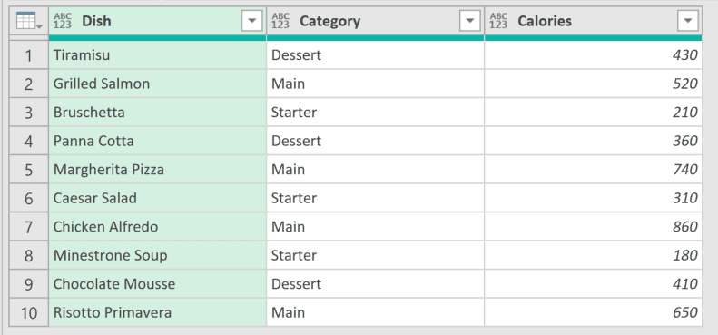
2. With a cell in the table selected, go to the Data tab and click From Table/Range. The Power Query Editor opens.

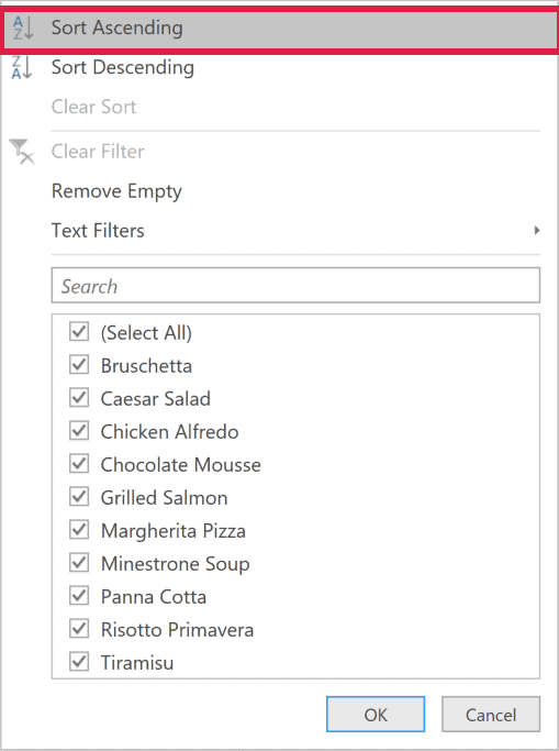
3. Click the dropdown arrow in the Dish column header and choose Sort Ascending.

4. Go to the Home tab in the editor, click Close & Load, and Excel drops the sorted result into a new table on a new sheet.

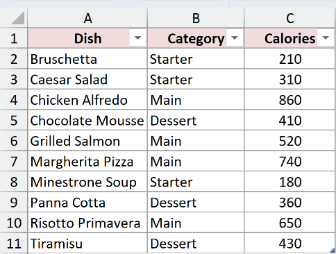
The new table lists every dish in A-to-Z order, with its category and calories intact. Your original data stays put on its own sheet.

Note: Power Query does not update on its own. When the source data changes, right-click the loaded table and choose Refresh, or click Refresh All on the Data tab, to re-sort with the new rows.

Method #6: Using VBA

If sorting is one step inside a bigger routine you run often, a short VBA macro can do it for you.

The Range.Sort method sorts a range alphabetically in a single line, so you can wire it into a larger automated process.

Here is the menu list the macro will sort by dish name.

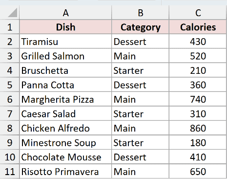
Here is the VBA code:

Sub SortDishesAtoZ()
    Dim ws As Worksheet
    Set ws = ThisWorkbook.Worksheets("VBA Sort")
    ws.Range("A1:C11").Sort Key1:=ws.Range("A2"), _
        Order1:=xlAscending, Header:=xlYes, Orientation:=xlTopToBottom
End Sub

Sub SortDishesAtoZ()
    Dim ws As Worksheet
    Set ws = ThisWorkbook.Worksheets("VBA Sort")
    ws.Range("A1:C11").Sort Key1:=ws.Range("A2"), _
        Order1:=xlAscending, Header:=xlYes, Orientation:=xlTopToBottom
End Sub

Here are the steps to run this macro:

1. In Windows, press Alt + F11 to open the Visual Basic Editor. On a Mac, choose Developer > Visual Basic.

2. Click Insert, then Module, and paste the code into the module window.

3. Press F5 to run the macro, then switch back to the worksheet.

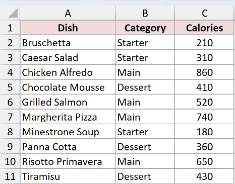
The macro sorts A1:C11 on the VBA Sort worksheet in the workbook that contains the macro.

Every Range reference uses ws, so activating a different sheet cannot redirect the sort.

Key1 points to the Dish column, Order1 sets A-to-Z order, and Header:=xlYes keeps the header row out of the sort.

If your worksheet has a different name, change "VBA Sort" in the Set statement.

Note: Running a macro clears Excel’s undo history, so you can’t Ctrl + Z the sort afterward. Save a copy of the file before you run it, and save the workbook as a macro-enabled .xlsm file to keep the code.

Additional Notes About Sorting Alphabetically in Excel

• Excel’s sort ignores case by default, so “apple” and “Apple” are treated as equal for sorting. You can turn on case sensitivity in the Sort dialog under Options.
• Leading spaces push a value to the top of an A-to-Z sort because a space sorts before letters. Run Find and Replace or the TRIM function to clean stray spaces before sorting.
• Numbers stored as text sort character by character, so “100” lands before “20”. If a text-format column sorts oddly, convert it to real numbers first.
• Sorting is not linked to the source once done with a button or dialog. SORT updates automatically when its referenced data changes, while Power Query re-sorts only when you refresh the query.

Frequently Asked Questions

How do I sort alphabetically without messing up other columns?

Click one cell in the sort column inside the connected data range, then use the A to Z button or Sort dialog.

If Excel shows a Sort Warning, choose Expand the selection so each complete row moves together.

Can I sort alphabetically and ignore case sensitivity in Excel?

Yes, and case is ignored by default.

Excel treats uppercase and lowercase letters as the same when sorting, so you don’t have to do anything extra unless you want case to matter.

How do I sort by the last word in a cell alphabetically, such as a last name?

Excel sorts full names from the start of each cell, so they are normally ordered by first name.

In Microsoft 365 or Excel 2024, pull the final word into a helper column with =TEXTAFTER(TRIM(A2)," ",-1,,,TRIM(A2)), then sort by that column.

The fallback keeps a single-word value unchanged.

Conclusion

I’ve covered six ways to sort text alphabetically while keeping each row together, including built-in tools, SORT, Power Query, and VBA.

I hope you found this article helpful!

Other Excel articles you may also like:

• Table.Sort Function (Power Query M)
• How to Create Custom Lists in Excel?
• How to Sort by Length in Excel? (Formula)
• How to Sort a Pivot Table in Excel?
• Reorder Rows in Pivot Table in Excel