
If you want the rows in a table reordered based on the values in one column, sorting by column is what you need. It sounds simple, but sort the wrong way and the other columns get scrambled.
The good news is that Excel keeps every column together as long as you sort the table the right way. In this article I’ll show you five easy ways to sort by column: the quick sort buttons, the Sort dialog box, the filter drop-down, a multi-level sort, and the SORT function.
Method #1: Using the Quick Sort Buttons
The fastest way to sort by column is the pair of A-Z and Z-A buttons on the Data tab.
You click one cell in the column you care about, hit a button, and the whole table reorders around that column. This is the one I reach for when the column to sort by is obvious.
Below I have a set of survey responses. Each row has a Response ID, the respondent’s name, the question they rated, and a Rating from 1 to 5. I want to sort the rows so the highest ratings sit at the top.
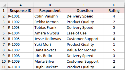
Here are the steps to sort by the Rating column with the quick sort buttons:
- Click any single cell inside the Rating column (for example, D2).
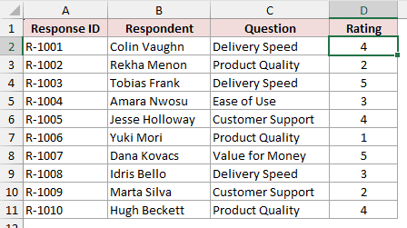
Note: Click a single cell, not the whole column. If you select just the Rating column, Excel shows a Sort Warning. Choose Expand the selection to keep each row intact. Choosing Continue with the current selection sorts only the ratings and moves them out of line with the names.
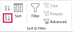
- On the Data tab, in the Sort & Filter group, click the Z to A button. With a column of numbers this sorts largest to smallest.
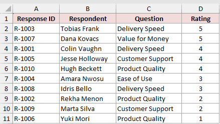
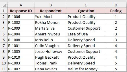
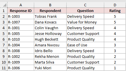
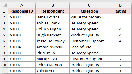
Excel instantly reorders the rows so the 5-star ratings are on top and the 1-star rating is at the bottom. Every respondent stays attached to their own rating and question.
If you want the opposite order, click the A to Z button instead. For a number column that sorts smallest to largest, so the 1-star response moves to the top.
Method #2: Using the Sort Dialog Box
If you’d rather pick the exact column by name, the Sort dialog box is for you.
It’s the better choice when several columns look alike, when your data has no headers, or when you want to line up more than one sort level. You choose the column from a drop-down instead of clicking inside it.
I’m using the same survey table: Response ID, Respondent, Question, and a Rating from 1 to 5. This time I’ll pick the Rating column by name in the dialog and sort it largest to smallest.
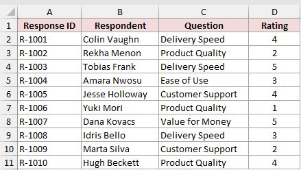
Here are the steps to sort by the Rating column using the Sort dialog box:
- Click any cell inside the data.
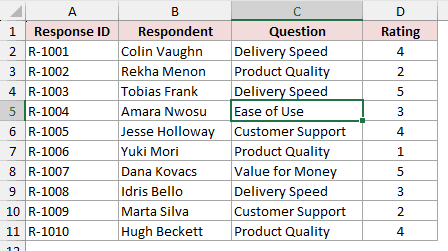
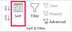
- On the Data tab, click Sort to open the Sort dialog box.
- Make sure the My data has headers box is checked so the header row stays on top.
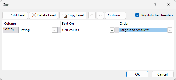
- In the Sort by drop-down, choose Rating. Leave Sort On set to Cell Values, and set Order to Largest to Smallest.
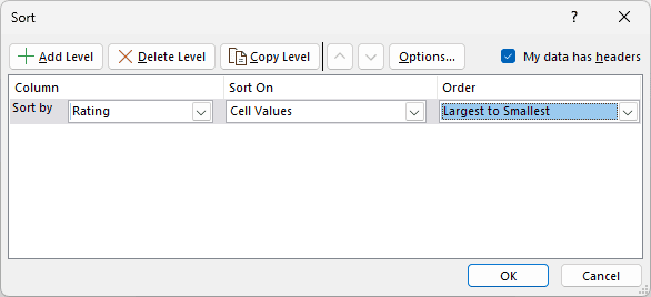
- Click OK.
The rows reorder by Rating, highest first, with each name and question kept next to its own rating.
Note: You can reach the same dialog from Home > Sort & Filter > Custom Sort, or by right-clicking a cell and choosing Sort > Custom Sort. All three open the same Sort box, so use whichever is closest.
Method #3: Using the Filter Drop-Down
If your table already has filter buttons on the header row, you never have to leave it. Every filter drop-down carries the sort commands right at the top.
This is the one to reach for when you are already filtering and just want the rows reordered without opening another dialog.
I’m using the same survey table: Response ID, Respondent, Question, and a Rating from 1 to 5. I want the highest ratings on top again, this time straight from the header row.
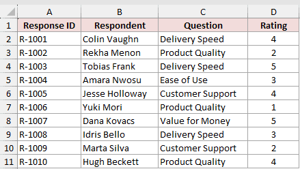
Here are the steps to sort by the Rating column from the filter drop-down:
- Click any cell inside the data, then on the Data tab click Filter to add the drop-down arrows to the header row.
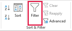
- Click the drop-down arrow on the Rating header.
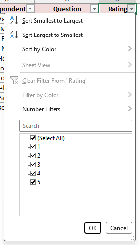
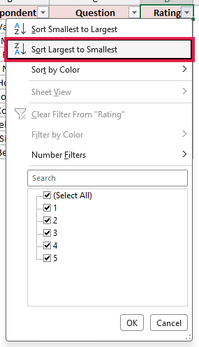
- Choose Sort Largest to Smallest.
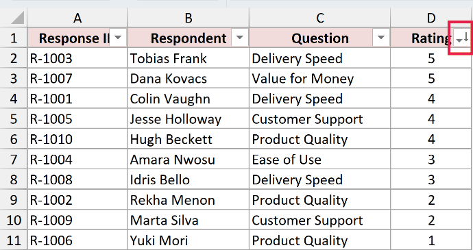
The rows reorder straight away, and a small arrow appears on the Rating button so you can tell at a glance which column the table is sorted by.
Note: The drop-down names the sort commands after the data type in that column. A text column offers Sort A to Z, a number column offers Sort Smallest to Largest, and a date column offers Sort Oldest to Newest. They are all doing the same job.
Method #4: Using a Multi-Level Sort
One column often isn’t enough. When several rows share the same value, you need a second column to settle the order inside each group.
The Sort dialog handles that with sort levels. The first level does the main ordering, and each level below it breaks the ties.
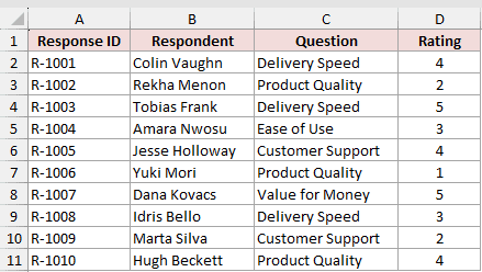
Here’s the same survey table. Three responses share a rating of 4 and two share a rating of 3, so I’ll sort by Rating largest to smallest first, then by Respondent A to Z inside each rating.
Here are the steps to run a two-level sort:
- Click any cell inside the data, then on the Data tab click Sort.
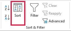
- With My data has headers checked, set Sort by to Rating and Order to Largest to Smallest.
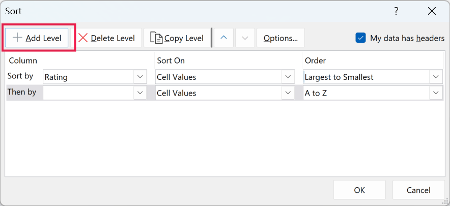
- Click Add Level to add a second row to the dialog.
- Set Then by to Respondent and leave Order as A to Z.
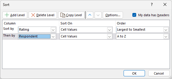
- Click OK.
The ratings now run from 5 down to 1, and inside the block of 4-star responses the names read Colin Vaughn, Hugh Beckett, Jesse Holloway in alphabetical order.
Note: The dialog’s other two drop-downs are worth knowing. Order holds a Custom List option for sequences Excel can’t guess, like High, Medium, Low. Sort On switches from Cell Values to Cell Color, Font Color, or Conditional Formatting Icon when you want to sort by how cells look rather than what they hold.
Method #5: Using the SORT Function
Every method above rearranges your actual data. If you’d rather leave the original table untouched and get a sorted copy somewhere else, the SORT function is the one to use.
It takes a range, sorts it by whichever column you name, and spills a fresh sorted range into empty cells.
Here’s the same survey table in A1:D11. I’ll place the formula in an empty cell to the right and get a sorted copy without changing the source.
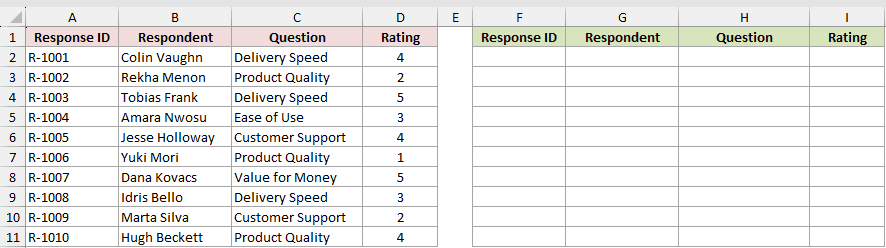
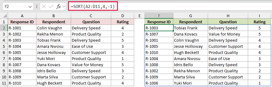
Here is the formula:
=SORT(A2:D11,4,-1)
How does this formula work?
SORT takes the array, the column to sort by, and the direction. I’m passing the data range A2:D11, then 4 for the sort index, then -1 for the order.
The sort index counts columns inside the array, so 4 points at Rating, the fourth column in A2:D11. The order -1 sorts largest to smallest. Use 1 instead if you want smallest to largest.
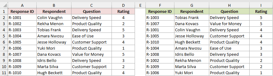
The result spills down automatically from the cell where you type the formula, so you only enter it once.
Because the range starts at A2, the header row isn’t included. If you want headers above the sorted copy, just type them in the row above the formula.
Note: SORT is available in Excel for Microsoft 365 and Excel 2021 and later. In older versions the function doesn’t exist and you’ll get a #NAME? error, so use one of the earlier methods instead.
Additional Notes About Sorting by Column in Excel
- Keep a stable ID column, like Response ID, in your data. After a sort scrambles the row order, you can sort by that column to get back to the original sequence.
- Sorting with the buttons or the dialog changes your data in place. If you might need the original order later, add an ID column first or work on a copy.
- To sort left to right instead of top to bottom, open the Sort dialog, click Options, and choose Sort left to right. The SORT function does the same with a fourth argument set to TRUE.
- Numbers stored as text won’t sort as numbers. If a rating column sorts oddly, convert those cells to real numbers first.
- Sorting only part of a table can misalign rows. Let Excel select the whole table by clicking one cell before you sort.
- Excel refuses to sort a range that contains merged cells. Unmerge them first, or the sort stops with a message telling you all merged cells need to be the same size.
Frequently Asked Questions
How do I sort by column instead of by row in Excel?
Sorting by column means reordering rows based on one column’s values, which is the default. Click a cell in that column and use the A-Z or Z-A button, or pick the column in the Sort dialog.
Why does sorting one column mess up the rest of my data?
That happens when you select a single column and choose to continue with just that selection. Excel then sorts that column alone and leaves the others in place. Click one cell instead so Excel sorts the entire table together.
Can I sort left to right across columns instead of down the rows?
Yes. Open the Sort dialog, click Options, and choose Sort left to right. Excel will then reorder your columns based on the values in a chosen row.
How do I sort by two columns at once in Excel?
Open the Sort dialog, set your first column, then click Add Level and pick the second one. Excel sorts by the top level first and uses each level below it to break ties. Method #4 walks through it.
Does the SORT function change my original data?
No. SORT returns a sorted copy in a new location and leaves the source range exactly as it is. That makes it handy when you need both the original order and a sorted view.
Conclusion
Sorting by column in Excel comes down to a handful of routes: the quick A-Z and Z-A buttons for a fast reorder, the Sort dialog box or the filter drop-down when you want to pick the column by name, a multi-level sort when one column leaves ties to settle, and the SORT function when you need a sorted copy that leaves the original alone.
For most jobs, the quick sort buttons are the fastest way to get there.
Other Excel articles you may also like:
